Brian O’Neill has held the City Council seat for the Northeast’s District 10 since 1980. He’s the lone Republican in a Council District seat, in addition to the two Republicans who hold the reserved At Large seats.
After running unopposed in 2015, O’Neill is being challenged this November by Democratic candidate Judy Moore.
Could he lose?
In the the surprising Primary in West Philly’s District 3, the cohorts that would decide the race were clear. In District 10, it’s harder to say. Is O’Neill a beloved incumbent whose ability to cross party lines will ensure his victory? Or have all elections become nationalized, dooming even a city-level official in Philadelphia’s most Republican (but still Democratic) neighborhoods?
District 10
District 10 covers the farthest sections of the Northeast, stretching down to Fox Chase and Rhawnhurt.
View code
library(tidyverse)
library(sf)
library(ggmap)
source("../../admin_scripts/util.R")

sf_council <- st_read("../../data/gis/city_council/Council_Districts_2016.shp")sf_divs <- st_read("../../data/gis/2019/Political_Divisions.shp")df <- readRDS("../../data/processed_data/df_all_2019_09_05.Rds")
df <- df %>%
  group_by(year, election, office, district, candidate, party, warddiv19) %>%
  summarise(votes=sum(votes)) %>%
  ungroup() %>%
  mutate(party = ifelse(party == "DEMOCRAT", "DEMOCRATIC", party))

bb <- st_bbox(sf_council %>% filter(DISTRICT == "10"))

expand_bb <- function(x, factor){
  mean_x <- mean(x)
  return(mean_x + factor * (x - mean_x))
}

bb[c(1,3)] <- expand_bb(bb[c(1,3)], 1.2)
bb[c(2,4)] <- expand_bb(bb[c(2,4)], 1.2)

names(bb) <- c("left", "bottom", "right", "top")
basemap <- get_map(location=bb, maptype="toner-lite")


get_labpt_df <- function(sf){
  df <- st_centroid(sf) %>%
    mutate(
      x=sapply(geometry, "[", 1),
      y=sapply(geometry, "[", 2)
    ) %>%
    as.data.frame() %>%
    select(-geometry)
  return(df)
}

phila_whole <- st_union(sf_council)

ggplot(sf_council) +
  geom_sf(data=phila_whole, fill="white", color=NA) +
  geom_sf(
    fill=strong_green, color = "white", size = 1, alpha=0.5
  ) +
  geom_sf(
    data=sf_council %>% filter(DISTRICT == "10"),
    fill=strong_green, color = "white", size = 1
  ) +
  geom_text(
    data = get_labpt_df(sf_council),
    aes(x=x,y=y,label=DISTRICT)
  ) +
  ggtitle("Philadelphia Council Districts") +
  theme_map_sixtysix()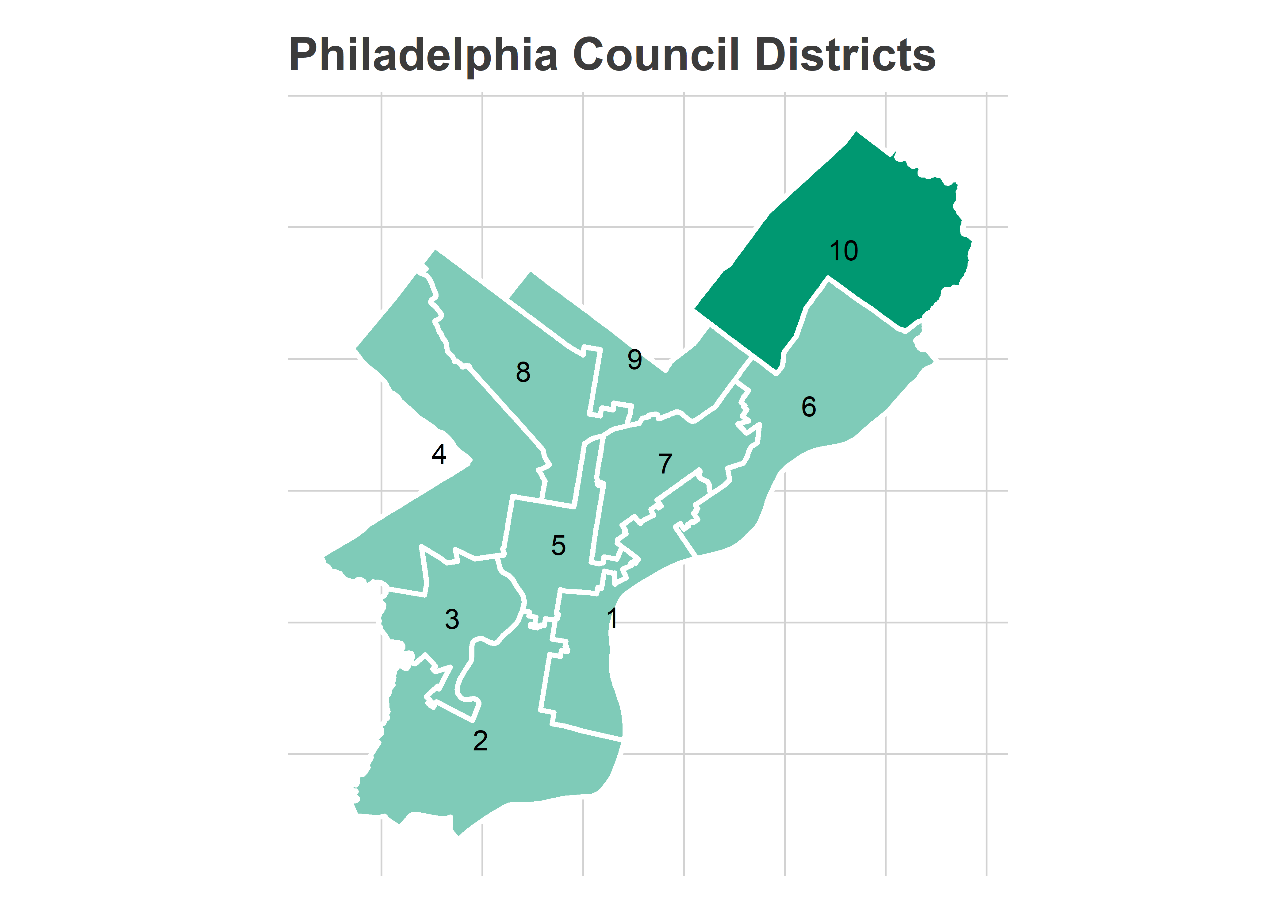
View code
district_map <- ggmap(
  basemap,
  extent="device",
  base_layer = ggplot(sf_council),
  maprange = FALSE
) +
  theme_map_sixtysix()

sf_divs$council_district <- sf_divs %>%
  st_centroid() %>%
  st_covered_by(sf_council) %>%
  (function(x){sf_council$DISTRICT[unlist(x)]})

district_map +
  geom_sf(
    aes(alpha = (DISTRICT == "10")),
    fill="black",
    color = "grey50",
    size=2
  ) +
  scale_alpha_manual(values = c(`TRUE` = 0.2, `FALSE` = 0), guide = FALSE) +
  ggtitle(sprintf("Council District %s", 10))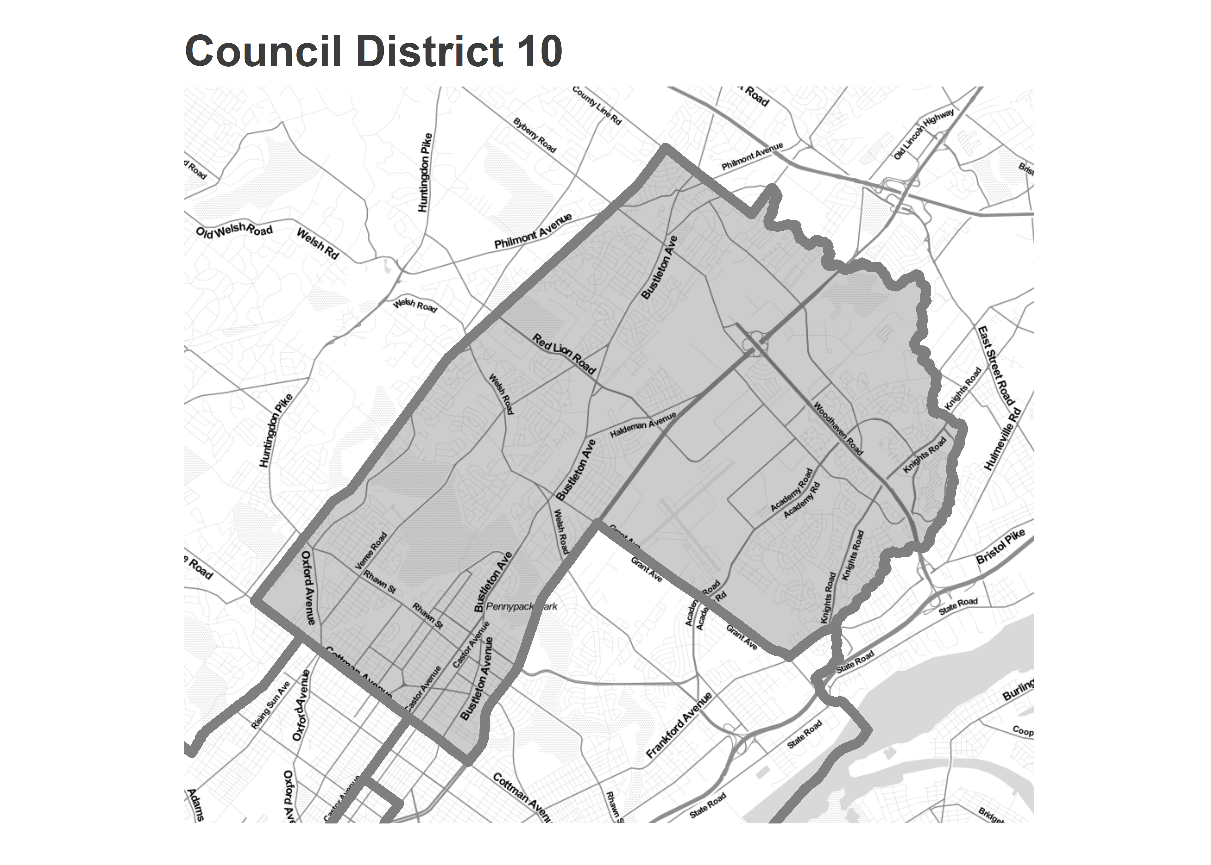
The district is consistently Philadelphia’s most Republican. It voted the most strongly for Trump (though Clinton still won overall), and is home to PA State Legislative District 170, represented by Republican Martina White.
(You can find all of these election maps, in interactive form, at the Ward Portal!)
View code
races <- tribble(
~election, ~office, ~district, ~short_office,
"general", "PRESIDENT OF THE UNITED STATES", NA, "President",
"general", "GOVERNOR", NA, "Governor",
"general", "REPRESENTATIVE IN CONGRESS", "2", "US Congress District 2",
"general", "MAYOR", NA, "Mayor"
# "2018", "general", "SENATOR IN THE GENERAL ASSEMBLY-2ND DISTRICT", "PA Senate"
)
candidate_votes <- df %>%
inner_join(races) %>%
group_by(warddiv19, short_office, year, election) %>%
mutate(
total_votes = sum(votes),
pvote = votes / sum(votes)
) %>%
group_by()
candidates_overall <- candidate_votes %>%
group_by(short_office, year, election, candidate, party) %>%
summarise(votes = sum(votes)) %>%
group_by(short_office, year, election) %>%
mutate(
pvote = votes/sum(votes),
use = pvote > 0.05
) %>%
filter(use)
candidate_votes <- candidate_votes %>%
inner_join(candidates_overall %>% select(year, election, short_office, candidate))
div_winners <- candidate_votes %>%
group_by(year, election, short_office, warddiv19) %>%
summarise(
winner = candidate[which.max(votes)],
winner_party = party[which.max(votes)],
winner_pvote = pvote[which.max(votes)],
twoparty_pvote = pvote[which.max(votes)] /
sum(pvote[party %in% c("DEMOCRATIC", "REPUBLICAN")], na.rm=TRUE),
total_votes = total_votes[1]
)
sf_divs <- sf_divs %>% rename(warddiv19 = DIVISION_N)
sf_divs$in_bbox <- sapply(
sf_divs$geometry,
function(g) {
coords <- as.matrix(g)
any(
coords[,1] > bb["left"] &
coords[,1] < bb["right"] &
coords[,2] > bb["bottom"] &
coords[,2] < bb["top"]
)
}
)
ggraces <- sf_divs %>%
filter(in_bbox) %>%
left_join(div_winners) %>%
mutate(
winner_party = format_name(substr(winner_party,1,3)),
race=sprintf("%s (%s)", short_office, year)
) %>%
mutate(race=factor(race, levels=unique(race[order(year)])))
district_map +
geom_sf(data=phila_whole, fill="white", color=NA) +
geom_sf(
data=ggraces %>% filter(year %in% c(2015, 2016, 2018)),
aes(fill = winner_party, alpha=100 * 2 * (twoparty_pvote - 0.5)),
color=NA
) +
geom_sf(
data=sf_council %>% filter(DISTRICT == "10"),
fill=NA,
color="white",
size=1
)+
facet_wrap(~race) +
scale_fill_manual(NULL, values=c("Dem"=strong_blue, "Rep"=strong_red)) +
theme_map_sixtysix() %+replace%
theme(legend.position = "bottom", legend.direction = "horizontal") +
scale_alpha_continuous("Win Margin (%)") +
guides(alpha = guide_legend(override.aes = list(fill = strong_blue)))+
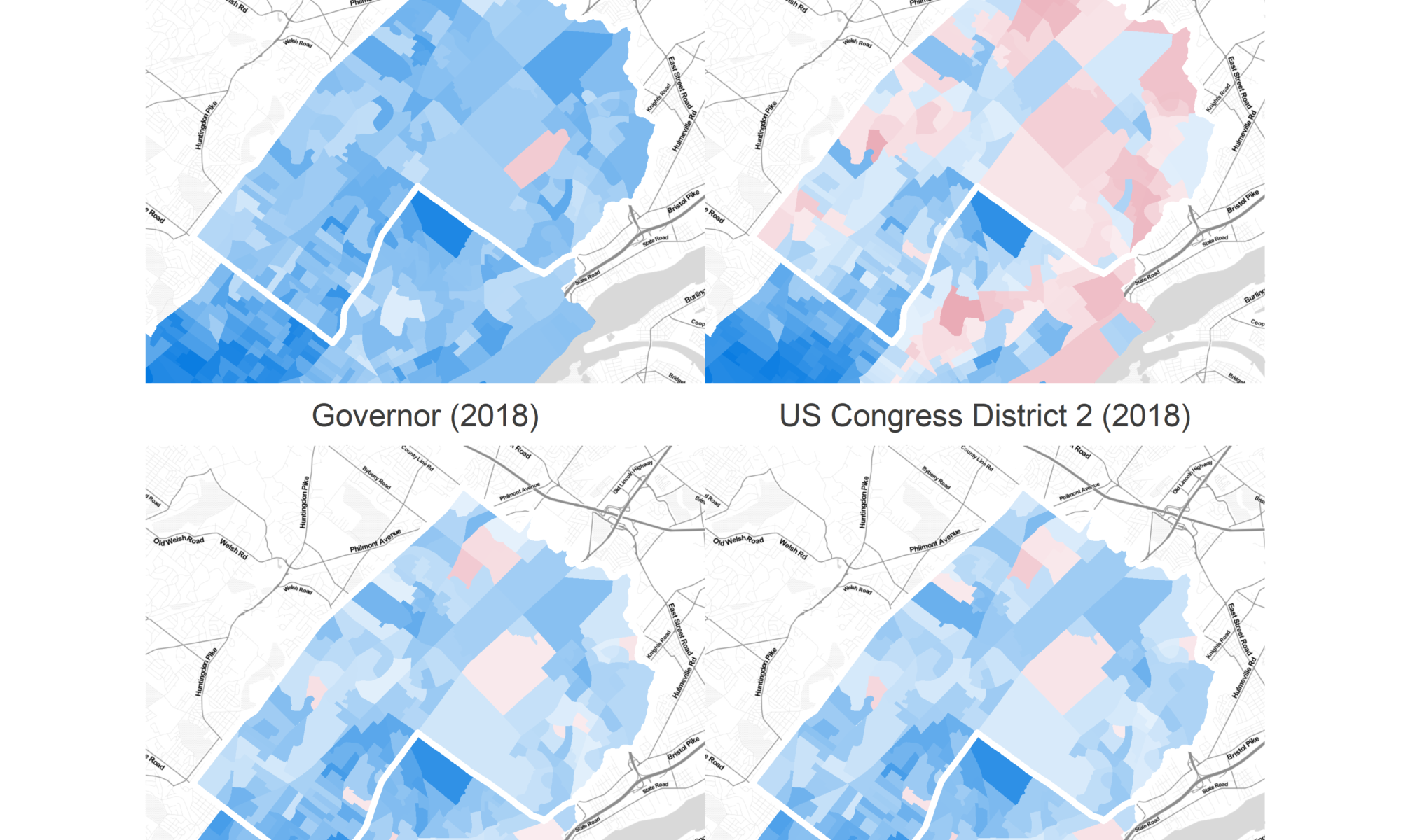
ggtitle("District 10's recent elections")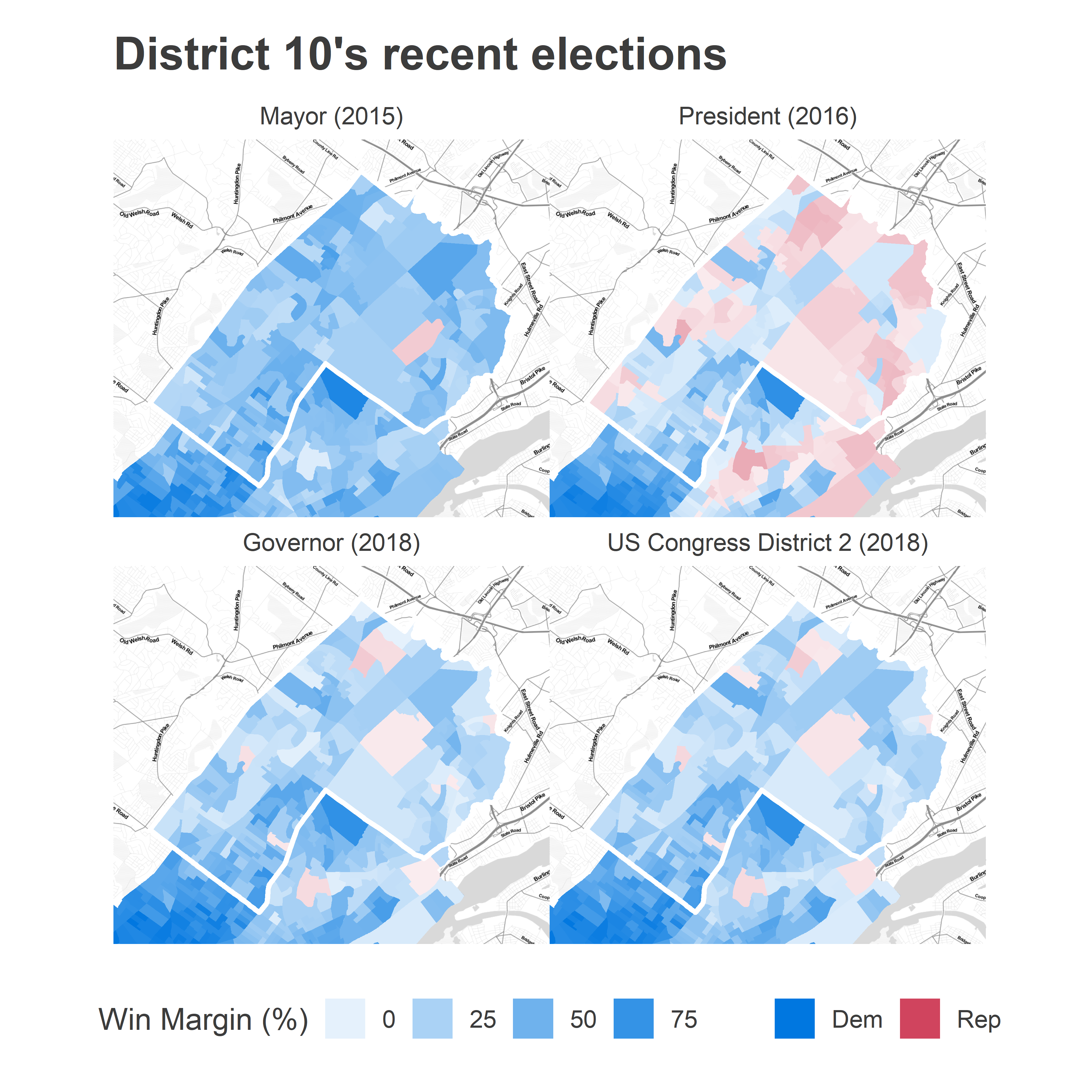
View code
sth_re <- "REPRESENTATIVE IN THE GENERAL ASSEMBLY"
sth_candidates <- df %>%
  filter(
    year == "2018", election=="general",
    office == sth_re
  ) %>%
  mutate(
    party=format_name(substr(party,1,3))
  ) %>%
  group_by(warddiv19, district, year, election) %>%
  mutate(
    total_votes = sum(votes),
    pvote = votes / sum(votes)
  ) %>%
  group_by()

sth_div_winners <- sth_candidates %>%
  filter(party %in% c("Dem", "Rep")) %>%
  group_by(year, election, district, warddiv19) %>%
  summarise(
    winner = candidate[which.max(votes)],
    winner_party = party[which.max(votes)],
    winner_pvote = pvote[which.max(votes)],
    twoparty_pvote = pvote[which.max(votes)] / sum(pvote)
  )

sf_sth <- st_read("../../data/gis/state_house/PaHouse2017_01.shp")sth_labpts <- sf_divs %>%
  filter(in_bbox) %>%
  left_join(sth_div_winners) %>%
  group_by(district) %>%
  dplyr::do(data.frame(geometry = st_union(.$geometry))) %>%
  ungroup() %>%
  mutate(geometry = st_sfc(geometry)) %>%
  st_as_sf() %>%
  get_labpt_df()

sth_labpts[sth_labpts$district=="170", c('x','y')] <- c(-75.02, 40.111)
sth_labpts[sth_labpts$district=="172", c('x','y')] <- c(-75.07, 40.079)
sth_labpts[sth_labpts$district=="173", c('x','y')] <- c(-75.002, 40.096)

district_map +
  geom_sf(data=phila_whole, fill="white", color=NA) +
  geom_sf(
    data=sf_divs %>%
      filter(in_bbox) %>%
      left_join(sth_div_winners),
    aes(fill = winner_party, alpha=100 * 2 * (twoparty_pvote - 0.5)),
    color=NA
  ) +
  geom_sf(
    data=sf_sth, fill=NA, color="black"
  ) +
  geom_sf(
    data=sf_council %>% filter(DISTRICT == "10"),
    fill=NA,
    color=rgb(1,1,1,0.8),
    size=2
  )+
  geom_text(
    data=sth_labpts,
    aes(x=x,y=y, label=district)
  )+
  scale_fill_manual(NULL, values=c("Dem"=strong_blue, "Rep"=strong_red)) +
  theme_map_sixtysix() %+replace%
  theme(legend.position = "bottom", legend.direction = "horizontal") +
  scale_alpha_continuous("Win Margin (%)") +
  guides(alpha = guide_legend(override.aes = list(fill = strong_blue)))+
  ggtitle("District 10's 2018 PA House elections")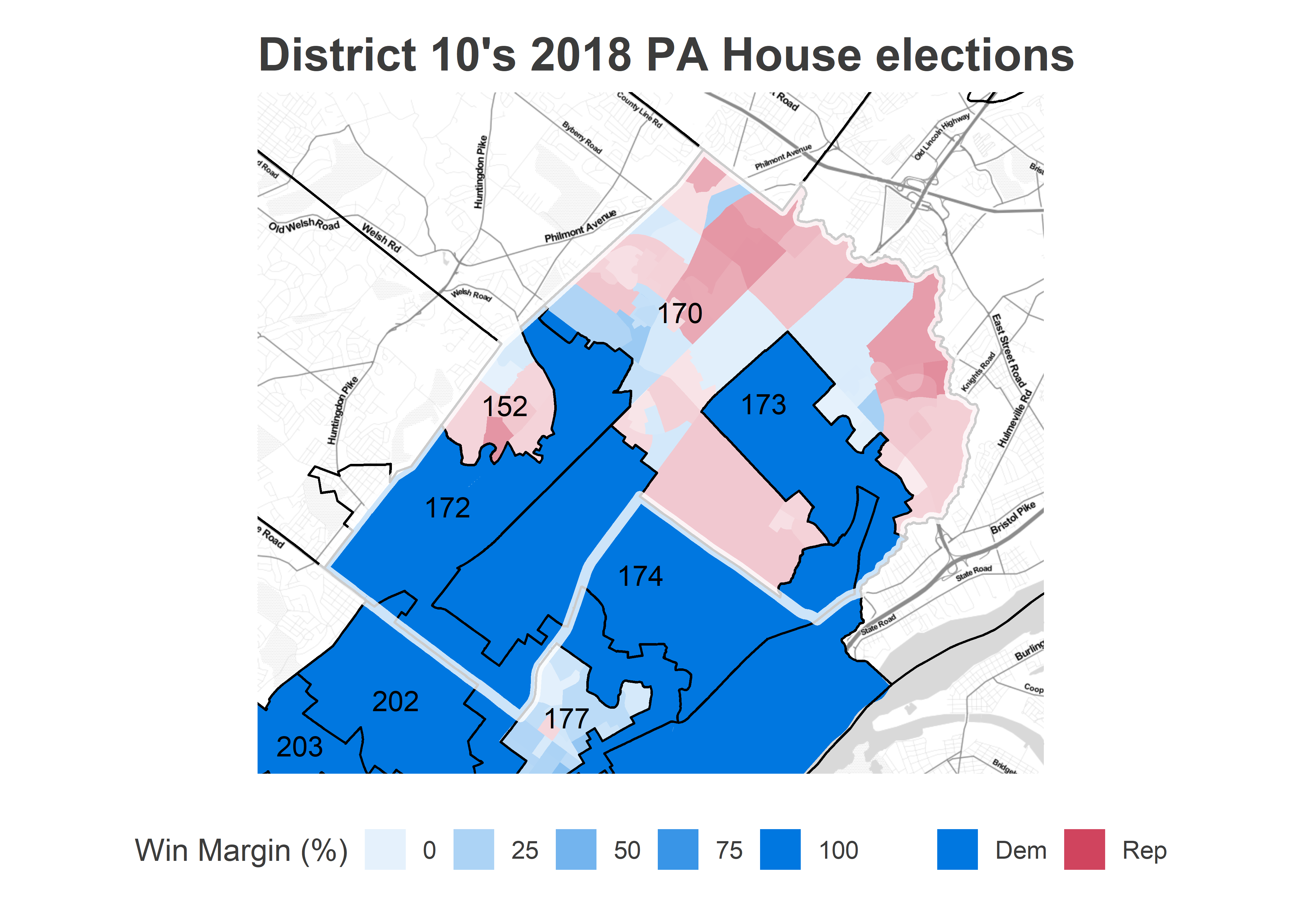
Many of the State House races were won by unopposed Democrats, with the two exceptions being Martina White’s 170, and the nub of Montgomery County’s 152. This makes it hard to project these races onto the District 10 race: how would those 100% districts have voted if there were a contest? There’s a big difference between if they would have gone 70% Democratic or 90%.
Recent races have varied in how divisive and how nationalized they were. In 2015, Kenney won broadly. The correlation between his performance and Clinton’s performance one year later was surprisingly weak. He won the district by 34 points, versus Clinton’s 5 point win, and won Divisions that Clinton lost handily.
View code
d10_scatter <- div_winners %>%
  inner_join(sf_divs %>% filter(council_district == "10")) %>%
  unite("office", short_office, year) %>%
  mutate(
    pdem_twoparty = ifelse(winner_party == "DEMOCRATIC", twoparty_pvote, 1-twoparty_pvote),
    win_gap = 2 * 100 * (pdem_twoparty-0.5)
  ) %>%
  select(office, warddiv19, win_gap, total_votes) %>%
  gather("key", "value", win_gap, total_votes) %>%
  unite(key, office, key) %>%
  spread(key, value)

gap_labeller <- function(x){
  sprintf(
    "%s%s%%%s",
    ifelse(x==0, "", "+"),
    abs(x),
    ifelse(x>0, " D", ifelse(x<0, " R", ""))
  )
}

plot_scatter <- function(col, office, title){
  col <- enquo(col)
  ggplot(
    d10_scatter,
    aes(x=President_2016_win_gap, y=!!col)
  ) +
    geom_abline(slope=1, intercept=0, linetype="dashed") +
    geom_hline(yintercept=0, color="black") +
    geom_vline(xintercept=0, color="black") +
    geom_point(aes(size = President_2016_total_votes), alpha = 0.3, pch = 16) +
    coord_fixed() +
    theme_sixtysix() %+replace%
    theme(legend.position = "right", legend.direction="vertical") +
    scale_size_area("Votes in 2016") +
    scale_x_continuous(
      "Win Gap for President (2016)",
      labels=gap_labeller
    )+
    scale_y_continuous(
      sprintf("Win Gap for %s", office),
      labels=gap_labeller
    ) +
    ggtitle(title, "Division-level results")
}

plot_scatter(Mayor_2015_win_gap, "Mayor (2015)", "Kenney was popular even in Trump's Divisions")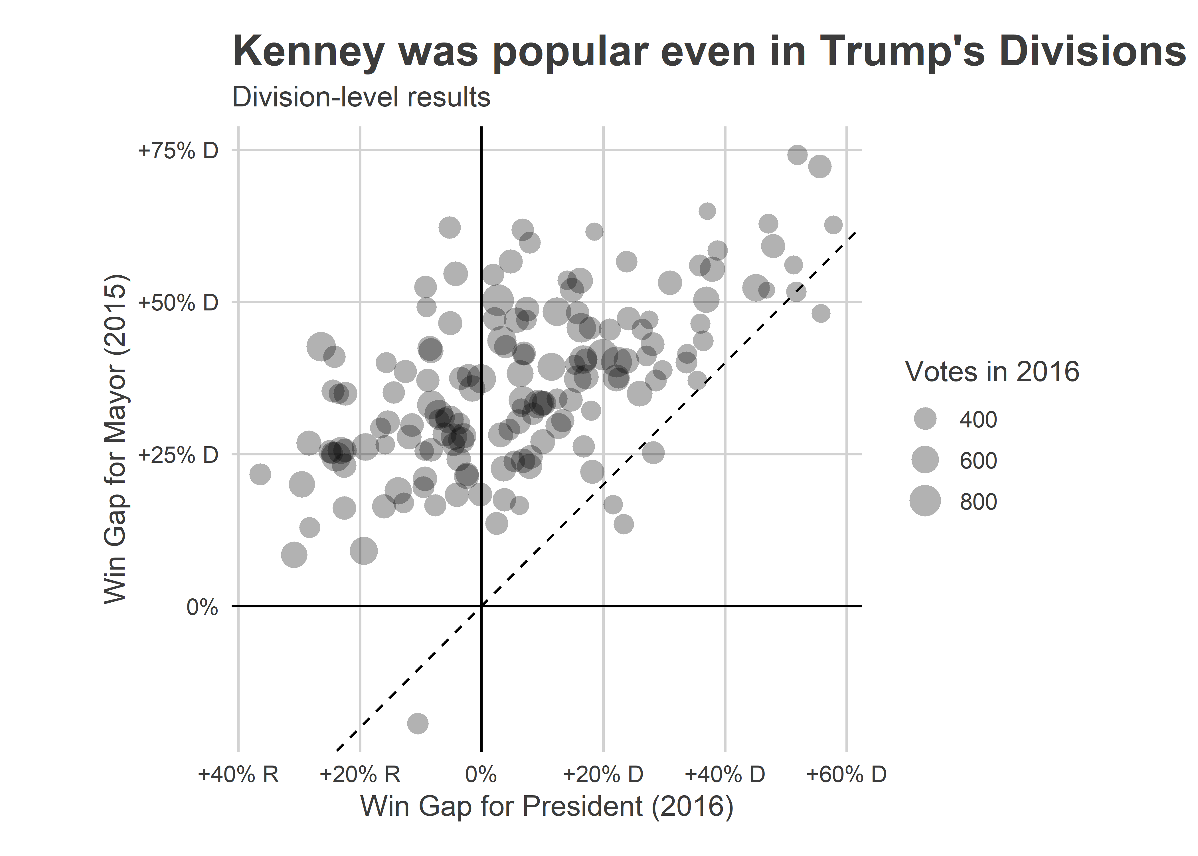
In comparison, Brendan Boyle’s 24-point win was much more correlated with Clinton. I interpret this as the race being nationalized, with party affiliation becoming salient. The main question for November is if O’Neill is a Kenney-esque candidate, who transcends party and Northeasters will continue to support, or if all elections are nationalized in a post-2016 world.
View code
plot_scatter(`US Congress District 2_2018_win_gap`, "US Congress District 2 (2018)", "Boyle won a nationalized race")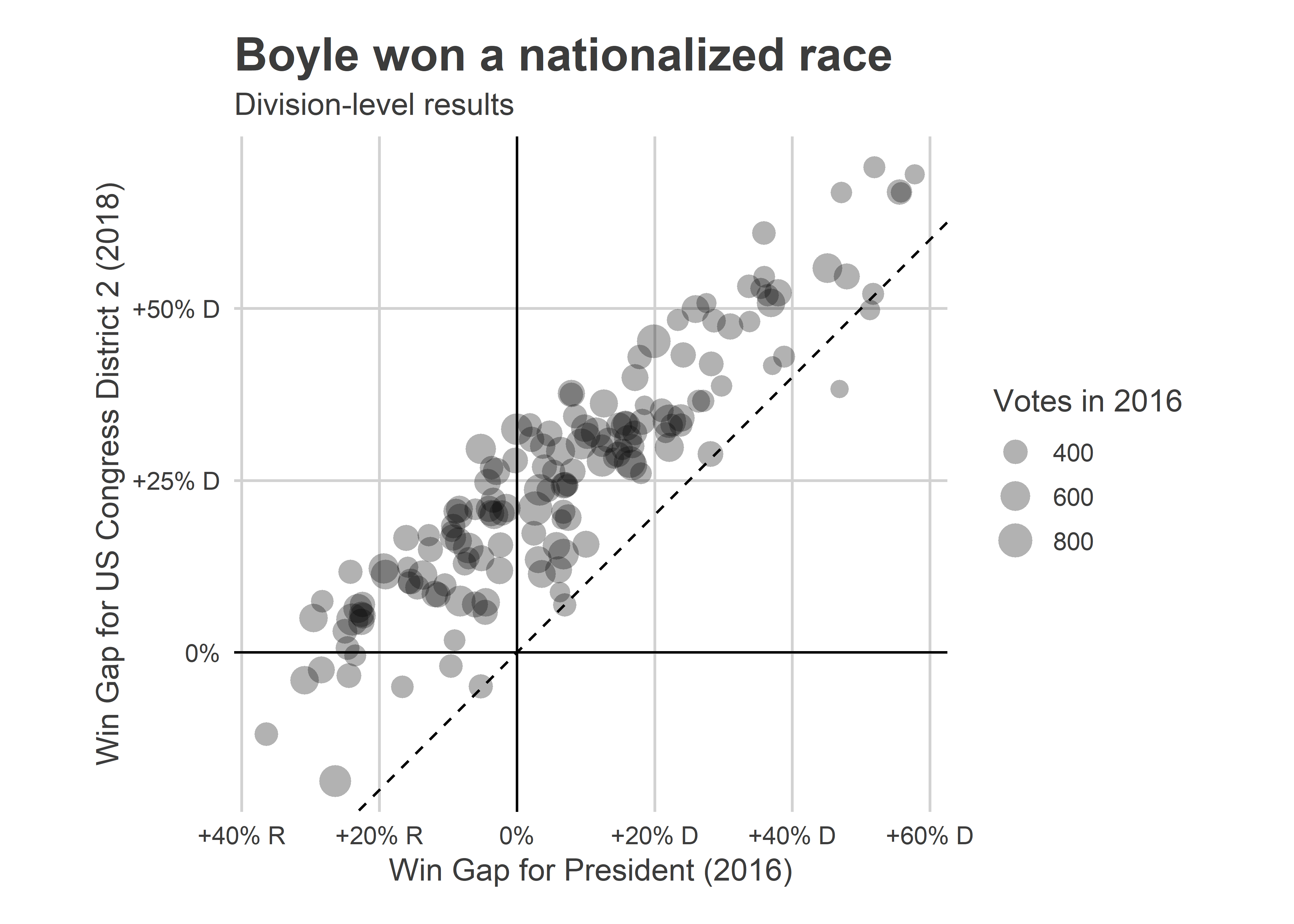
The challenge for Moore is that O’Neill consistenty runs ahead of every other Republican in the district.
Since 2003, there have been 21 uncontested District Council races. Only one of those was a Republican: O’Neill himself in 2015. So there’s not any history of uncontested Republicans to gain insights from.
View code
council <- df %>%
  filter(election == "general") %>%
  filter(office == "DISTRICT COUNCIL")

council_totals <- council %>%
  filter(candidate != "Write In") %>%
  filter(party %in% c("DEMOCRATIC", "REPUBLICAN")) %>%
  group_by(year, candidate, party, district) %>%
  summarise(votes=sum(votes)) %>%
  mutate(is_competitive = votes > 100) %>%
  group_by(year, district) %>%
  summarise(
    n_contested = sum(is_competitive),
    winner = candidate[which.max(votes)],
    winner_pct = votes[which.max(votes)] / sum(votes),
    winner_party = party[which.max(votes)]
  )

## council_totals %>% filter(winner_pct == 1)

oneill_df <- council_totals %>%
  filter(district == 10) %>%
  mutate(office = "Council", short_office="Council District 10") %>%
  rename(prep = winner_pct) %>%
  select(year, prep, short_office) %>%
  bind_rows(
    df %>%
      filter(
        office %in% c("MAYOR", "PRESIDENT OF THE UNITED STATES", "GOVERNOR"),
        election == "general",
        party %in% c("DEMOCRATIC", "REPUBLICAN")
      ) %>%
      mutate(short_office = format_name(office)) %>%
      inner_join(sf_divs %>% as.data.frame() %>% filter(council_district == 10) %>% select(warddiv19)) %>%
      group_by(year, party, short_office) %>%
      summarise(votes = sum(votes)) %>%
      group_by(year, short_office) %>%
      summarise(
        prep = votes[party == "REPUBLICAN"] / sum(votes)
      )
  )

ggplot(
  oneill_df ,
  aes(x=asnum(year), y=2*100*(prep-0.5), color=short_office)
) +
  geom_hline(yintercept = 00, color="grey20") +
  geom_point(
    size=3
  ) +
  geom_line(
    aes(group=short_office),
    size=1
  ) +
  theme_sixtysix() +
  ylab("Percent for Republican") +
  geom_text(
    data=data.frame(
      year=2015.2, prep=c(0.30, 0.95, 0.55, 0.4), label=c("Mayor", "O'Neill", "President", "Governor"),
      short_office=c("Mayor", "Council District 10", "President of the United States", "Governor")
    ),
    hjust=0, fontface="bold",
    aes(label=label)
  ) +
  scale_color_manual(
    guide=FALSE,
    values=c(
      "Mayor"=light_blue,
      "Council District 10"=light_red,
      "President of the United States"=light_purple,
      "Governor"=light_green
    )
  )+
  xlab(NULL) +
  scale_x_continuous(breaks = seq(2003, 2015, 4)) +
  scale_y_continuous(labels=function(x) gap_labeller(-x)) +
  ggtitle("O'Neill runs far ahead of other Republicans")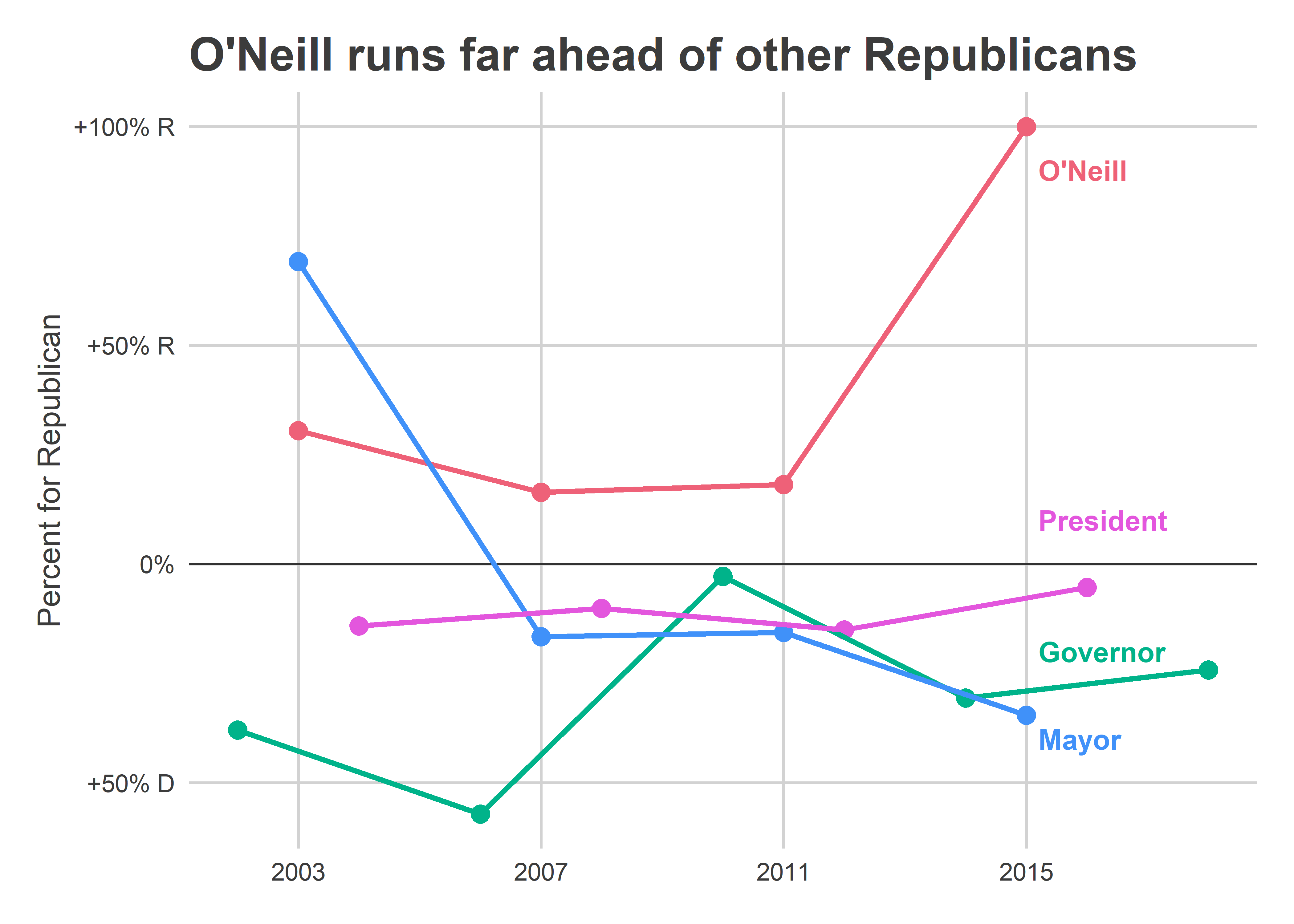
O’Neill ran 17 points ahead of the Republican candidate for Mayor in 2007 and 2011 (meaning a gap of 34 points). Then in 2015 he was unupposed. In thatDemocrats have won every single Presidential, Gubernatorial, and Mayoral race in the district since, with the only exception being voting for Katz over Street in 2003.
Comparative turnout in Municipal Elections
If the race becomes close, relative turnout of Republican and Democratic divisions might be decisive. The Republican divisions typically turn out more strongly in non-Presidential elections. Using turnout in 2016 as the baseline (my preferred method), very-Republican divisions had nearly 1.5 the relative turnout of the very-Democratic ones in 2015.
View code
turnout <- df %>% filter(
  election=="general",
  year %in% 2015:2018,
  office %in% c("MAYOR", "GOVERNOR", "PRESIDENT OF THE UNITED STATES", "DISTRICT ATTORNEY")
) %>%
  group_by(year, warddiv19) %>%
  summarise(turnout=sum(votes))

turnout <- sf_divs %>%
  as.data.frame() %>%
  select(warddiv19, Shape__Are) %>%
  left_join(turnout) %>%
  group_by(year) %>%
  mutate(
    turnout_per_area = turnout / Shape__Are,
    turnout_per_area_std = (
      turnout_per_area - mean(turnout_per_area)
    ) / sd(turnout_per_area)
  )

turnout_wide <- turnout %>%
  select(-turnout_per_area_std) %>%
  gather("key", "value", turnout, turnout_per_area) %>%
  unite("key", key, year) %>%
  spread(key, value) %>%
  inner_join(sf_divs %>% as.data.frame() %>% filter(council_district == "10") %>% select(warddiv19))

turnout_scatter <- function(year, title){
  turnout_col <- sym(paste0("turnout_", year))
  ggplot(
    turnout_wide %>% left_join(d10_scatter),
    aes(
      x=President_2016_win_gap,
      y=100*!!turnout_col / turnout_2016
    )
  ) +
    geom_point(
      aes(size=President_2016_total_votes),
      alpha = 0.5, pch=16
    ) +
    theme_sixtysix() +
    geom_smooth(
      aes(weight=President_2016_total_votes),
      color = "black", method=lm
    ) +
    scale_y_continuous(
      sprintf("Votes in %s / Votes in 2016 (%%)", year),
      breaks=seq(0,100,10)
    )+
    scale_x_continuous(
      "Win Gap for President (2016)",
      labels=gap_labeller
    ) +
    scale_size_area("Votes in 2016") +
    expand_limits(y=0) +
    ggtitle(title)
}

turnout_scatter(2015, "Republican Divisions voted disproportionately\n in 2015")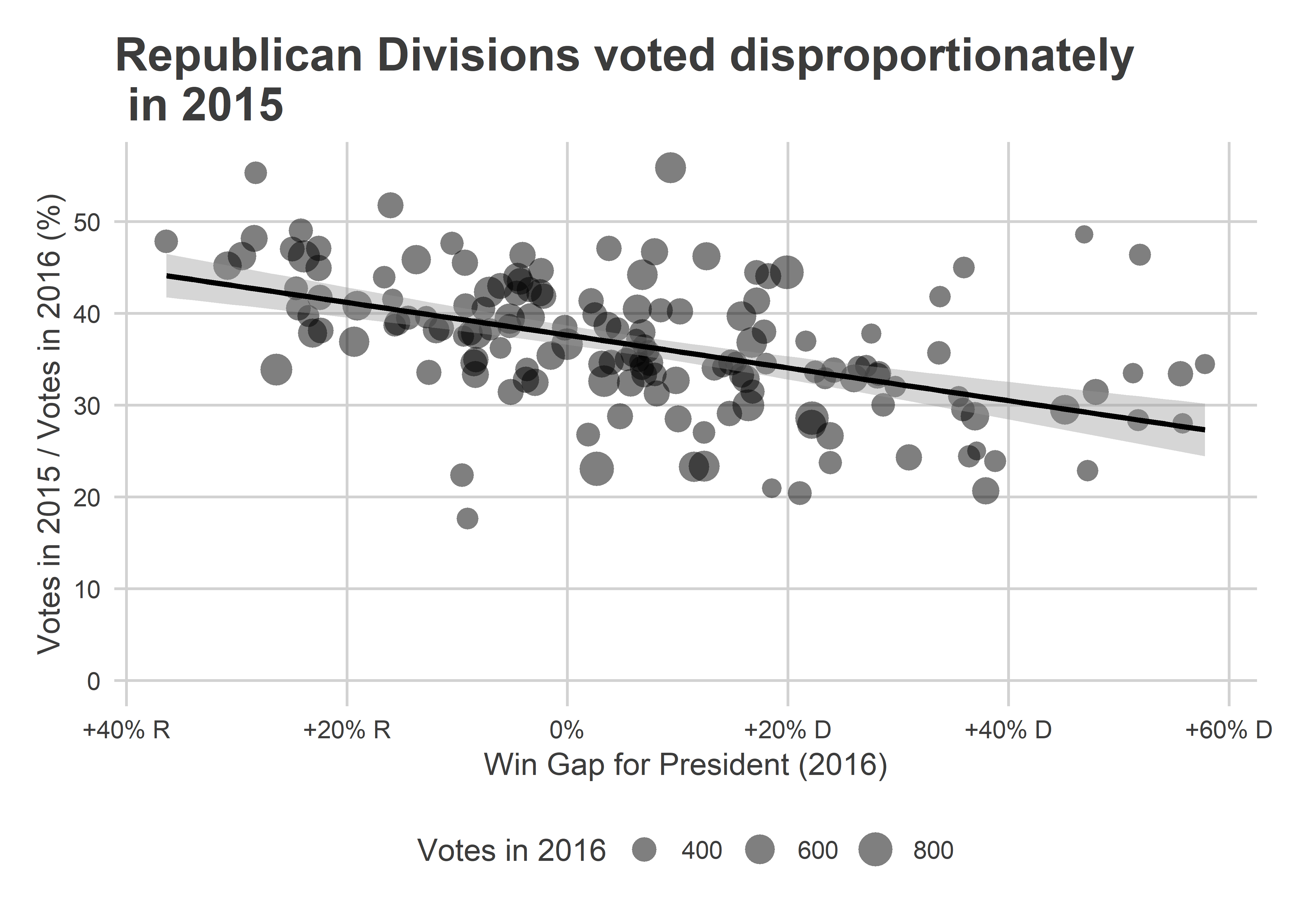
That changed in 2018. The gap was still about ten percentage points, but at a much higher overall level. Republicans’ proportional advantage was significantly weakened.
View code
turnout_scatter(2018, "Republican Divisions had less turnout advantage\n in 2018")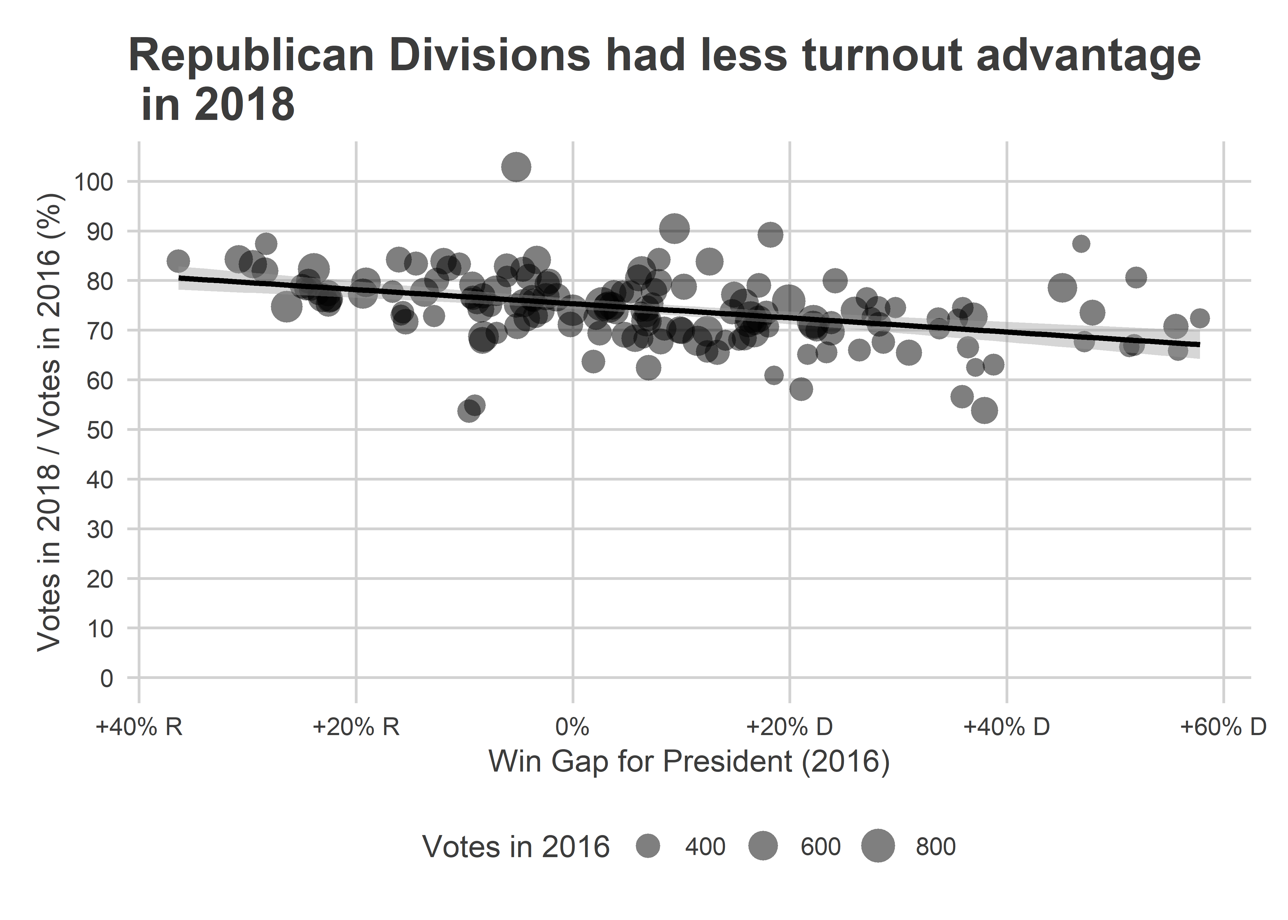
How many votes is the turnout difference between 2015 and 2018 worth? Using the division results from 2016, but turnout from 2015 and 2018, the difference between 2015 and 2018 would have been a gap of 1.2 for the Democrat. Not enough to change the results in all but the closest of races.
View code
turnout_wide %>%
  left_join(d10_scatter) %>%
  summarise(
    gap_2015=weighted.mean(President_2016_win_gap, w=turnout_2015),
    gap_2016=weighted.mean(President_2016_win_gap, w=turnout_2016),
    gap_2018=weighted.mean(President_2016_win_gap, w=turnout_2018)
  )
## # A tibble: 1 x 3
## gap_2015 gap_2016 gap_2018
## <dbl> <dbl> <dbl>
## 1 3.44 5.35 4.60Moore needs to hope that even City Council has become nationalized.
Really the only way Moore can win is if the divisions that regularly vote for Democrats, the divisions that carried Kenney and Clinton and Boyle to victory, turn against O’Neill. This is increasingly happening across the country, but O’Neill has a big cushion.
Maybe, just maybe, Boyle’s decisive 2018 win was a sign of a changing district. The only way to know for sure would be polling. Without that, we’ll see in November.