Pennsylvania elects our judges, but really they win by a lottery. The order of the candidates on the ballot is determined by names out of a can, and for a Common Pleas candidate, getting your name in the first column nearly triples your votes.
The easiest way to eliminate this unearned benefit is to change the order of candidates across the city. If you’re at the top of the ballot in one place, you should be at the bottom of the ballot elsewhere. Candidates would then still get the benefit of ballot position whenever their name was in the first column, but that effect would be spread across all the candidates, instead of to the same candidate on every single ballot. The result would be that other factors, almost certainly more correlated with candidate quality, would determine the winner.
I had heard that implementing different ballots to different parts of the city would require a change to the state election code. But there are whispers that the letter of the law might actually allow for Philadelphia to use different orders. (I can’t find an online source, but believe me, there are whispers).
I’m not a lawyer, so can’t speak to whether the argument is legitimate. I am a data scientist, so can explore the next questions: if we could randomize ballot position, how should we do it? And would it really help?
Analytic strategy
I am going to simulate recent elections using different strategies for reordering the ballot.
Five ballot order methods
Let’s consider five methods for arranging the ballot.
- Status Quo: Randomly generate a single order of the candidates, and use that order in every Division
- Randomize all Divisions: Randomly generate a new candidate order for each Division. This is probably the gold standard, and would reduce the ballot-order effect to near zero. I don’t think this is a bad ask; we already print unique ballots for each precinct, and it shouldn’t be too hard to re-order a race for each (especially as we buy new-fangled machines).
- Randomize Wards: Randomly generate a candidate order for each Ward, and use that for all Divisions within the Ward. People seem more comfortable with this option than randomizing by Division, even though to me it seems like an unnecessary second-best.
- The Wheel: Randomize the order of candidates in one ward, and then cycle through the order in the other wards, so that every candidate is guaranteed to be in the top spot the same fraction of wards. I’ll use “the Wheel”, a way to strategically resort candidates to minimize the ballot position effect.
- The California Cycle: Randomize the order of candidates in the 1st Ward, then shift them one position for each next ward. Similar to the Wheel, but less strategic. A version of this system has been the law in California elections since 1975.
Note: I’m not an election official, and have no idea if these proposals are possible on a given hardware or software that we use. It may be true that the machines have not been programmed to be capable of the randomizations above. I am willing to say that we live in the age of computers, and if our systems aren’t capable of these basic tasks, that’s dumb. California has randomized ballot order for state elections since 1975.
Running simulations
How should we simulate an election? It’s not obvious: you need to decide what features of past elections to leave intact, and what to randomize. Here’s my approach:
First: I will start with the Common Pleas Division-level results. I’ll subtract out the effect of the ballot order, using Ward-specific estimates for ballot position effects, to create order-corrected Division results. This will leave intact the effect of DCC endorsements, Bar recommendations, campaign spending, and division-level preferences. I’ll be re-calculating only the effect of the ordering.
Second: For each method, I then simulate the candidate order 400 times. For each of these orders I will add on the effect of the new ballot position (using Ward-specific effects).
(Note: The Ward-specific effects were obviously calculated under the elections we have. Adding on these Status Quo estimates of position effects will almost certainly overstate the importance of ballot position in the new methods; the new methods will probably lessen the effect of ballot position even within Divisions. My current estimates combine the fact that voters push buttons in the first column with the fact that candidates with good ballot position have an easier time fundraising and spend more time campaigning. In the randomized scenarios, only the first effect will operate within Divisions, and not the second. Thus, the new methods will probably be even better than what I predict here.)
Third: For each candidate order, I’ll simulate 100 elections by randomly drawing election results from a multinomial distribution for each precinct. This gives me a measure of the randomness within a given ordering (making 100,000 simulations per method per election). Then I can look across orderings for a measure of randomness due to the ordering itself.
Fourth: To evaluate a method, I’ll look at how often each candidate wins within a given ordering, compared to how often they win across orderings. If the method eliminates the effect of ballot position, then these numbers should be the same: candidates will win just as often for a given ordering as they do overall. If the randomness of the method still affects the results, then candidates will win more often for some orderings than they do overall. I’ll calculate the average of the absolute difference between the two, and call it the average absolute deviation due to ordering.
Mathematically, suppose for method \(m\), I simulate 400 orderings, \(o \in \{1,…,400\}\). For each ordering, I simulate 100 elections and measure the fraction of elections in which each candidate wins: \(p_{moc}\) is the fraction of times candidate \(c\) wins under ordering \(o\) in method \(m\).
\(\frac{1}{N_c N_o} \sum_c \sum_o |p_{moc} – \frac{1}{N_o}\sum_{o’}p_{mo’c}|\)
For example, if a candidate wins 20% of the time across all orderings, but ballot position matters so much that they win 100% of the time in 1/5 of orderings and 0% of the time in the other 4/5, they will contribute a \(0.2 \times |1.0 – 0.2| + 0.8 \times |0.0 – 0.2| = 0.32\) absolute deviation. If a candidate wins just as often for a given ordering as they do overall, they will contribute 0.0.
(This’ll be clear when we do some examples.)
The Status Quo
View code
library(ggplot2)
library(dplyr)
library(tidyr)
library(tibble)
library(readr)
library(forcats)
library(knitr)
library(kableExtra)
set.seed(215)
source("../../admin_scripts/util.R")
ballot <- read.csv("../../data/common_pleas/judicial_ballot_position.csv")
ballot$name <- tolower(ballot$name)
ballot$name <- gsub("[[:punct:]]", " ", ballot$name)
ballot$name <- trimws(ballot$name)
ballot$year <- as.character(ballot$year)
df_all <- safe_load("C:/Users/Jonathan Tannen/Dropbox/sixty_six/data/processed_data/df_all_2019_07_09.Rda")
df <- df_all %>%
filter(
election == "primary",
grepl("COMMON PLEAS$", OFFICE),
PARTY == "DEMOCRATIC",
CANDIDATE != "Write In",
year >= 2009
)
rm(df_all)
df <- df %>%
mutate(
CANDIDATE = tolower(CANDIDATE),
CANDIDATE = gsub("\\s+", " ", CANDIDATE)
) %>%
group_by(CANDIDATE, year, WARD19, DIV19) %>%
summarise(votes = sum(VOTES)) %>%
ungroup()
df_ward <- df %>%
group_by(CANDIDATE, year, WARD19) %>%
summarise(votes = sum(votes)) %>%
group_by(year, WARD19) %>%
mutate(pvote = votes / sum(votes)) %>%
ungroup
df_total <- df_ward %>%
group_by(year, CANDIDATE) %>%
summarise(votes = sum(votes))
election <- tibble(
year = as.character(c(2009, 2011, 2013, 2015, 2017, 2019)),
votefor = c(7, 10, 6, 12, 9, 6)
)
election <- election %>% left_join(
ballot %>%
mutate(year = as.character(year)) %>%
group_by(year) %>%
summarise(
nrows = max(rownumber),
ncols = max(colnumber),
ncand = n(),
n_philacomm = sum(philacommrec),
n_inq = sum(inq),
n_dcc = sum(dcc)
)
)
df_total <- df_total %>%
inner_join(election) %>%
group_by(year) %>%
arrange(desc(year), desc(votes)) %>%
mutate(finish = 1:n()) %>%
mutate(winner = finish <= votefor)
df_total <- df_total %>% inner_join(
ballot,
by = c("CANDIDATE" = "name", "year" = "year")
)
df_total <- df_total %>%
group_by(year) %>%
mutate(pvote = votes / sum(votes))
df <- df %>%
inner_join(ballot, by = c("CANDIDATE"="name", "year"="year"))
df_ward <- df_ward %>%
inner_join(ballot, by = c("CANDIDATE"="name", "year"="year"))
prep_data <- function(df){
df %>% mutate(
rownumber = fct_relevel(factor(as.character(rownumber)), "3"),
colnumber = fct_relevel(factor(as.character(colnumber)), "3"),
col1 = colnumber == 1,
col2 = colnumber == 2,
col3 = colnumber == 3,
row1 = rownumber == 1,
row2 = rownumber == 2,
col1row1 = (colnumber==1) & (rownumber==1),
col1row2 = (colnumber==1) & (rownumber==2),
is_rec = philacommrec > 0,
is_highly_rec = philacommrec==2,
inq=inq>0,
candidate_year = paste0(CANDIDATE, "::", year)
)
}
df_ward <- prep_data(df_ward)
df_ward <- df_ward %>%
group_by(year, WARD19) %>%
mutate(pvote = votes / sum(votes)) %>%
ungroup
library(lme4)
# better opt: https://github.com/lme4/lme4/issues/98
library(nloptr)
defaultControl <- list(
algorithm="NLOPT_LN_BOBYQA",xtol_rel=1e-6,maxeval=1e5
)
nloptwrap2 <- function(fn,par,lower,upper,control=list(),...) {
for (n in names(defaultControl))
if (is.null(control[[n]])) control[[n]] <- defaultControl[[n]]
res <- nloptr(x0=par,eval_f=fn,lb=lower,ub=upper,opts=control,...)
with(res,list(par=solution,
fval=objective,
feval=iterations,
conv=if (status>0) 0 else status,
message=message))
}
USE_SAVED <- TRUE
rfit_filename <- "outputs/lmer_fit.Rds"
if(!USE_SAVED){
rfit <- lmer(
log(pvote + 0.001) ~
(1 | candidate_year)+
col1row1 +
col1row2+
row1 + row2 +
I(gender == "F") +
col1 + col2 +
dcc +
is_rec + is_highly_rec +
factor(year) +
(
# row1 + row2 +
col1row1 +
col1row2 +
I(gender == "F") +
col1 + col2 + #col3 +
dcc +
is_rec + is_highly_rec
| WARD19
),
df_ward,
control=lmerControl(optimizer="nloptwrap2")
)
saveRDS(rfit, file=rfit_filename)
} else {
rfit <- readRDS(rfit_filename)
}
df_ward$fitted <- predict(rfit)
ranef <- as.data.frame(ranef(rfit)$WARD19) %>%
rownames_to_column("WARD19") %>%
gather("variable", "random_effect", -WARD19) %>%
mutate(
fixed_effect = fixef(rfit)[variable],
effect = random_effect + fixed_effect
)
ranef_wide <- ranef %>%
select(WARD19, variable, effect) %>%
spread(variable, effect)
df_pred <- df %>%
group_by(year, WARD19, DIV19) %>%
mutate(pvote = votes/sum(votes)) %>%
group_by() %>%
left_join(ranef_wide, by="WARD19") %>%
mutate(
log_pvote = log(pvote + 0.001)
) %>%
mutate(
log_pvote_adj = log_pvote -
ifelse(
colnumber == 1, col1TRUE, 0
) -
ifelse(
colnumber == 2, col2TRUE, 0
) -
ifelse(
colnumber == 1 & rownumber == 1, col1row1TRUE, 0
) -
ifelse(
colnumber == 1 & rownumber == 2, col1row2TRUE, 0
)
)
turnout <- df_pred %>% group_by(year, WARD19, DIV19) %>%
summarise(votes=sum(votes)) %>%
ungroup()
run_elections <- function(
df, year, order, nrow=11, ncol=3, n_elec=1e3
){
if(!all(c("CANDIDATE", "order") %in% colnames(order))){
stop(
"order should be a dataframe with columns CANDIDATE, order, and maybe WARD19 DIV19"
)
}
order <- order %>% mutate(
col = ((order-1) %/% nrow)+1,
row = order - (col-1)*nrow
)
## assume everything is correctly sorted
df$log_pvote <- df %>%
left_join(order) %>%
with(
log_pvote_adj +
ifelse(col==1, col1TRUE, 0) +
ifelse(col==2, col2TRUE, 0) +
ifelse(col==1 & row==1, col1row1TRUE, 0) +
ifelse(col==1 & row==2, col1row2TRUE, 0)
)
df$pvote <- exp(df$log_pvote)
votes <- df %>%
ungroup() %>%
select(CANDIDATE, WARD19, DIV19, pvote, turnout, year) %>%
mutate(expected_votes = pvote * turnout) %>%
group_by(CANDIDATE, year) %>%
summarise(expected_votes = sum(expected_votes)) %>%
ungroup() %>%
left_join(
expand.grid(year=as.character(year), elec=1:n_elec)
) %>%
mutate(
votes = rpois(n(), lambda=expected_votes)
)
return(votes %>% select(CANDIDATE, elec, votes))
}
run_sims <- function(
get_order_fn, year, df=df_pred, nsims=400,
nelec=1e2, verbose=TRUE,
return_orders=TRUE, return_results=TRUE
){
df <- df %>%
filter(year == !!year) %>%
arrange(WARD19, DIV19, CANDIDATE)
df <- df %>%
left_join(
turnout %>% filter(year == !!year) %>% rename(turnout=votes)
)
results <- vector(mode="list", length=nsims)
orders <- vector(mode="list", length=nsims)
win_fracs <- vector(mode="list", length=nsims)
for(i in 1:nsims){
order_sim <- get_order_fn(df) %>%
mutate(sim=i)
if(return_orders) orders[[i]] <- order_sim
result <- run_elections(
df, year, order_sim, n_elec=nelec
) %>% mutate(sim=i)
if(return_results) results[[i]] <- result
win_fracs[[i]] <- get_win_frac(result, year)
if(verbose) if(i %% 10 == 0) print(i)
}
return_list <- list(
win_fracs=bind_rows(win_fracs),
year=year
)
return_list$dev <- get_dev(return_list$win_fracs)
if(return_results) return_list$results <- bind_rows(results)
if(return_orders) return_list$orders <- bind_rows(orders)
return(return_list)
}
get_win_frac <- function(
results,
year
){
nwinners <- election$votefor[election$year == year]
results <- results %>%
group_by(sim, elec) %>%
mutate(
pvote = votes/sum(votes),
rank = rank(desc(votes), ties.method="first")
) %>%
ungroup() %>%
mutate(is_winner = (rank <= nwinners)) %>%
group_by(sim, CANDIDATE) %>%
summarise(
pwin = mean(is_winner),
pvote = mean(pvote)
)
return(results)
}
get_dev <- function(frac_winners){
frac_winners <- frac_winners %>%
group_by(CANDIDATE) %>%
summarise(
dev = mean(abs(pwin - mean(pwin))),
pwin = mean(pwin)
)
return(frac_winners)
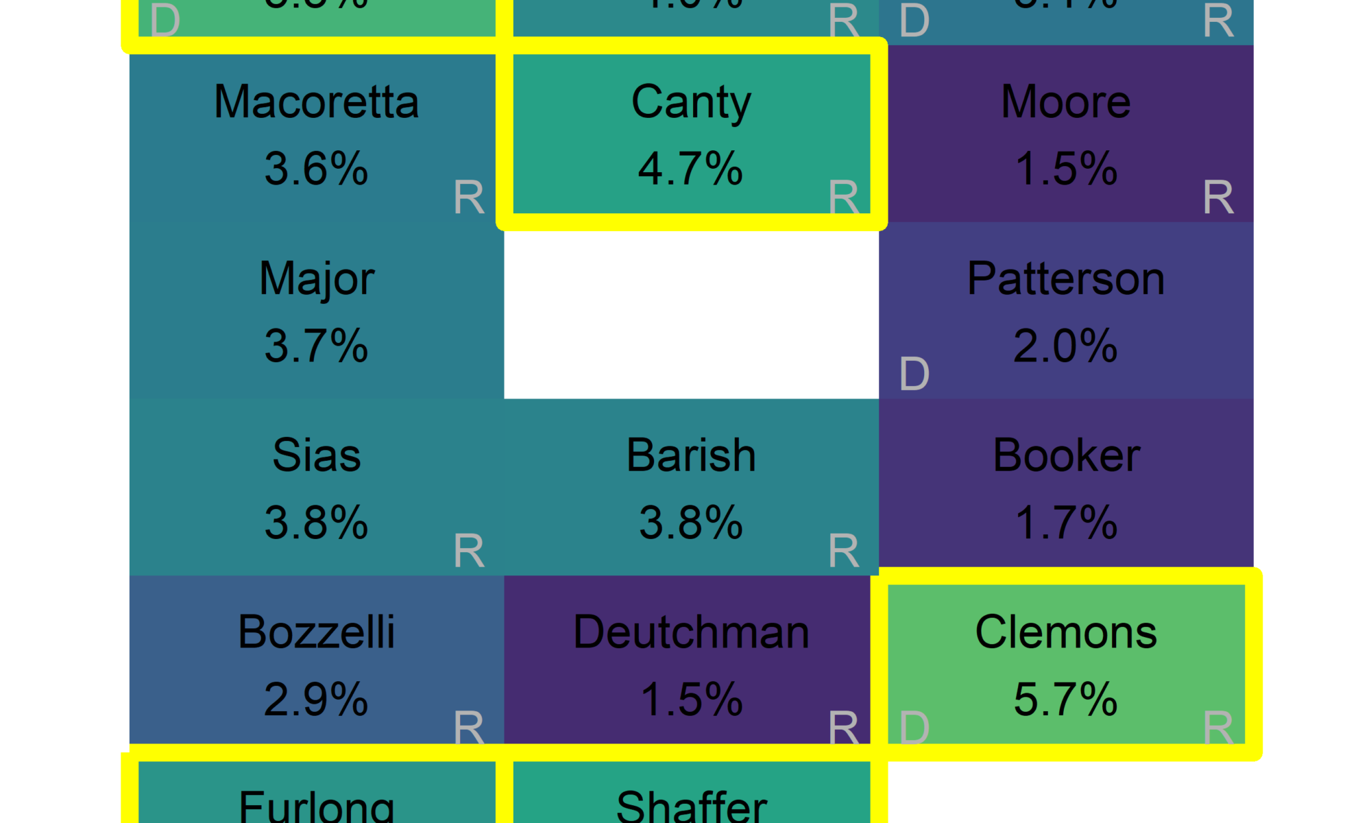
}First, consider the Status Quo: we randomly allocate the order once for the entire city.
In the actual 2017 election, six candidates from the first column won, including three Not Recommended candidates. Stella Tsai and Vikki Kristiansson came in 1 and 2, and were also the first and second listed on the ballot. Lucretia Clemons finished in third, from the third column and seventh row.
View code
ggplot(
  df_total %>%
    filter(year == 2017) %>%
    mutate(
      lastname=format_name(gsub(".*\\s(\\S+)$", "\\1", CANDIDATE))
    ) %>%
    arrange(votes),
  aes(y=rownumber, x=colnumber)
) +
  geom_tile(
    aes(fill=pvote*100, color=winner),
    size=2
  ) +
  geom_text(
    aes(
      label = ifelse(philacommrec==1, "R", ifelse(philacommrec==2,"HR","")),
      x=colnumber+0.45,
      y=rownumber+0.45
    ),
    color="grey70",
    hjust=1, vjust=0
  ) +
  geom_text(
    aes(
      label = ifelse(dcc==1, "D", ""),
      x=colnumber-0.45,
      y=rownumber+0.45
    ),
    color="grey70",
    hjust=0, vjust=0
  ) +
  geom_text(
    aes(label = sprintf("%s\n%0.1f%%", lastname, 100*pvote)),
    color="black"
    # fontface="bold"
  ) +
  scale_y_reverse(NULL) +
  scale_x_continuous(NULL)+
  scale_fill_viridis_c(guide=FALSE) +
  scale_color_manual(values=c(`FALSE`=NA, `TRUE`="yellow"), guide=FALSE) +
  annotate(
    "text",
    label="R = Recommended\nD = DCC Endorsed",
    x = 1.6,
    y = 11,
    hjust=0,
    color="grey70"
  ) +
  expand_limits(x=3.5)+
  theme_sixtysix() %+replace%
  theme(
    panel.grid.major=element_blank(),
    axis.text=element_blank()
  ) +
  ggtitle(
    "2017 Common Pleas Results",
    "Democratic Primary. Winners are outlined."
  )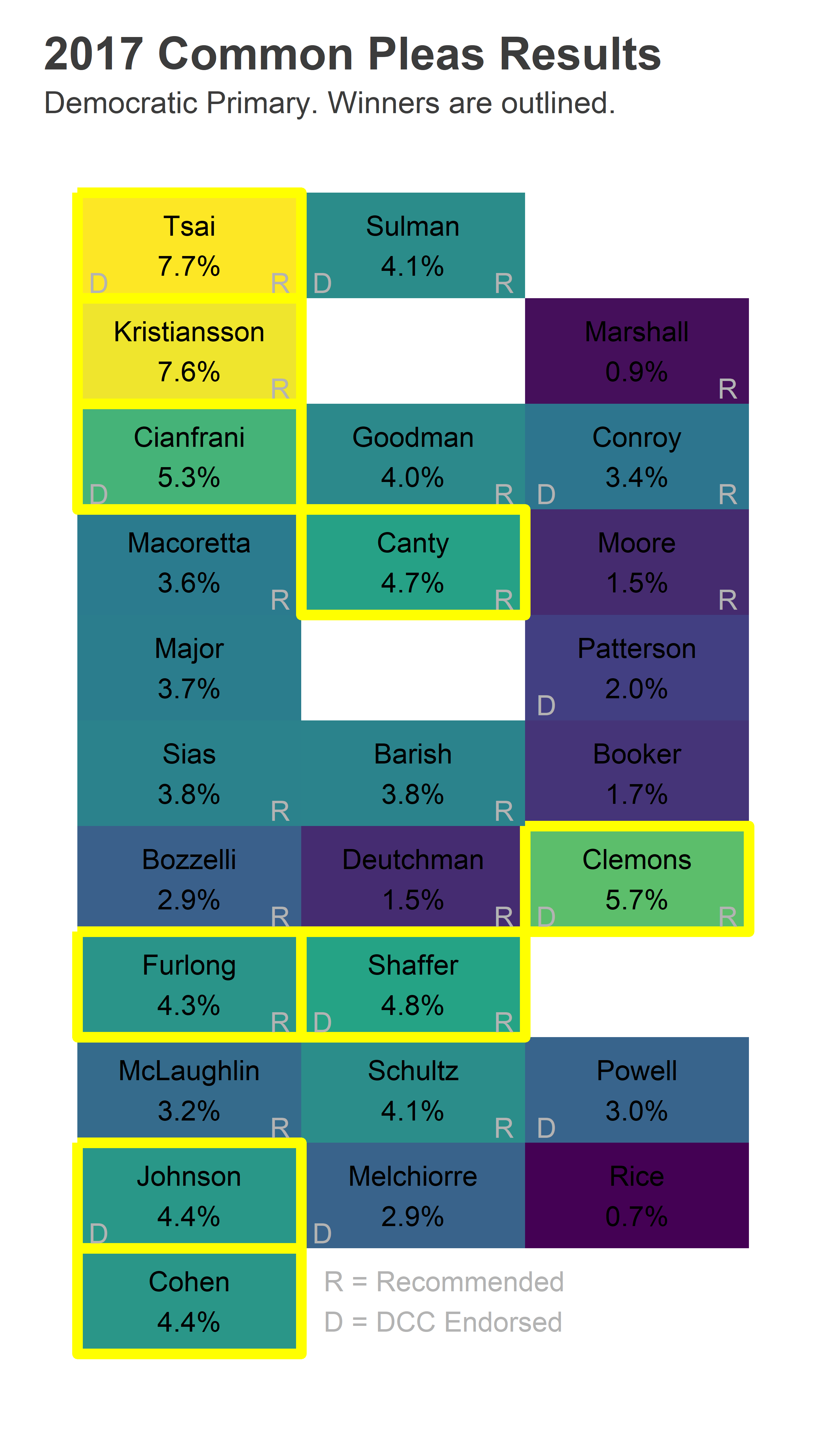
What would have happened if we re-randomized the order? Clemons almost certainly would still win: she won out of the third column, and a new lottery could only help. Tsai and Kristiansson had positions that typically receive a 3x bump; in the third column we would expect them to have only received about 2.5%, not enough for a win.
We can simulate those results.
Status Quo Simulations
View code
set.seed(215)
status_quo_order <- function(df){
  cands <- unique(df$CANDIDATE)
  order <- sample.int(length(cands))
  return(
    data.frame(CANDIDATE=cands, order=order)
  )
}

status_quo_results <- run_sims(
  status_quo_order, 2017, nsims=1e2, nelec=1e2, verbose=FALSE
)
To understand what’s happening, let’s look at the first simulation. Here are the eleven candidates in the first column:
View code
status_quo_results$orders %>%
  filter(sim==1) %>%
  arrange(order) %>%
  with(as.character(CANDIDATE[1:11]))
## [1] "leonard deutchman" "mark j moore" "jennifer schultz"
## [4] "crystal b powell" "henry mcgregor sias" "vincent melchiorre"
## [7] "lucretia c clemons" "stella tsai" "leon goodman"
## [10] "brian mclaughlin" "jon marshall"Leonard Dutchman got the top position, Mark More second. Stella Tsai still managed the first column, but in 8th place instead of first.
Among the elections with this order, the same 9 candidates won every time. This includes top vote-getter Lucretia Clemons; she did so well from the last column in the real 2017 election that when this lottery put her seventh, she won 12% of the vote.
Six of the winners came from the first column. Six were women, five were DCC-endorsed, and two were Not Recommended by the Bar.
View code
status_quo_results$orders %>%
  filter(sim==1) %>%
  inner_join(
    get_win_frac(status_quo_results$results, 2017)
  ) %>%
  arrange(desc(pvote)) %>%
  mutate(
    pvote=round(100*pvote),
    pwin=round(100*pwin, 1)
  ) %>%
  left_join(
    ballot %>% filter(year == 2017) %>%
      select(name, gender, philacommrec, dcc),
    by = c("CANDIDATE"="name")
  ) %>%
  `[`(1:11, c(-3)) %>%
  kable() %>%
kable_styling()| CANDIDATE | order | pwin | pvote | gender | philacommrec | dcc |
|---|---|---|---|---|---|---|
| lucretia c clemons | 7 | 100 | 12 | F | 1 | 1 |
| crystal b powell | 4 | 100 | 7 | F | 0 | 1 |
| leon goodman | 9 | 100 | 6 | M | 1 | 0 |
| jennifer schultz | 3 | 100 | 6 | F | 1 | 0 |
| stella tsai | 8 | 100 | 5 | F | 1 | 1 |
| zac shaffer | 19 | 100 | 4 | M | 1 | 1 |
| vikki kristiansson | 15 | 100 | 4 | F | 1 | 0 |
| deborah canty | 20 | 100 | 4 | F | 1 | 0 |
| vincent melchiorre | 6 | 100 | 4 | M | 0 | 1 |
| daniel r sulman | 22 | 0 | 4 | M | 1 | 1 |
| mark j moore | 2 | 0 | 4 | M | 1 | 0 |
How about across all simulations, including re-orderings?
View code
summary_table <- function(results){
  table <- get_win_frac(results$results, results$year) %>%
    group_by(CANDIDATE) %>%
    summarise(pwin = mean(pwin), pvote=mean(pvote)) %>%
    arrange(desc(pwin), desc(pvote)) %>%
    mutate(
      pvote=round(100*pvote, 1),
      pwin=round(100*pwin, 1)
    ) %>%
    left_join(
      ballot %>% filter(year == results$year) %>%
        select(name, gender, philacommrec, dcc),
      by = c("CANDIDATE"="name")
    ) %>%
    ungroup() %>%
    mutate(CANDIDATE=format_name(CANDIDATE)) %>%
    rename(
      Candidate=CANDIDATE,
      `Win %`=pwin,
      `Avg Vote %`=pvote,
      Gender=gender,
      `Bar Rec`=philacommrec,
      `DCC Endorsement`=dcc
    )

  kable(table) %>%
    kable_styling() %>%
    scroll_box(height="300px")
}

summary_stats <- function(results){
    results$win_fracs %>%
    group_by(CANDIDATE) %>%
    summarise(
      dev = mean(abs(pwin - mean(pwin))),
      pwin = mean(pwin),
      pvote=mean(pvote)
    ) %>%
    left_join(
      ballot %>% filter(year == results$year) %>%
        select(name, gender, philacommrec, dcc),
      by = c("CANDIDATE"="name")
    ) %>%
    group_by() %>%
    summarise(
      dev = mean(dev),
      n_rec = sum((philacommrec>0)*pwin),
      n_dcc = sum((dcc>0)*pwin)
    )
}

summary_table(status_quo_results) | Candidate | Win % | Avg Vote % | Gender | Bar Rec | DCC Endorsement |
|---|---|---|---|---|---|
| Lucretia C Clemons | 100.0 | 9.6 | F | 1 | 1 |
| Zac Shaffer | 83.3 | 5.2 | M | 1 | 1 |
| Deborah Canty | 83.1 | 5.4 | F | 1 | 0 |
| David Conroy | 80.0 | 5.9 | M | 1 | 1 |
| Crystal B Powell | 74.5 | 5.0 | F | 0 | 1 |
| Vikki Kristiansson | 74.1 | 4.9 | F | 1 | 0 |
| Jennifer Schultz | 60.1 | 4.8 | F | 1 | 0 |
| Stella Tsai | 42.0 | 4.1 | F | 1 | 1 |
| Daniel R Sulman | 40.0 | 4.2 | M | 1 | 1 |
| Deborah Cianfrani | 37.0 | 3.7 | F | 0 | 1 |
| Danyl S Patterson | 36.0 | 3.4 | F | 0 | 1 |
| Wendi Barish | 34.0 | 3.9 | F | 1 | 0 |
| Leon Goodman | 30.0 | 4.0 | M | 1 | 0 |
| Vincent Melchiorre | 27.9 | 3.3 | M | 0 | 1 |
| Shanese Johnson | 25.0 | 3.1 | F | 0 | 1 |
| Mark B Cohen | 20.1 | 3.2 | M | 0 | 0 |
| Terri M Booker | 18.9 | 3.0 | F | 0 | 0 |
| Vincent Furlong | 18.0 | 3.1 | M | 1 | 0 |
| Henry McGregor Sias | 5.0 | 2.9 | M | 1 | 0 |
| John Macoretta | 5.0 | 2.7 | M | 1 | 0 |
| Rania Major | 3.0 | 2.7 | F | 0 | 0 |
| Brian McLaughlin | 2.0 | 2.3 | M | 1 | 0 |
| Mark J Moore | 1.0 | 2.6 | M | 1 | 0 |
| Lawrence J Bozzelli | 0.0 | 2.2 | M | 1 | 0 |
| Leonard Deutchman | 0.0 | 1.7 | M | 1 | 0 |
| Jon Marshall | 0.0 | 1.6 | M | 1 | 0 |
| Bill Rice | 0.0 | 1.4 | M | 0 | 0 |
View code
# summary_stats(status_quo_results)Lucretia Clemons won in every simulation; she did so well in the real election that reordering can’t touch her.
Eight of the nine most frequent winners were Recommended by the Bar, though only 6.6 Recommended candidates win on average. How is that possible? That’s the problem with the lottery. It introduces additional randomness to a given simulation that means a few Not Recommended candidates will overperform their average performance, and win. That lucky winner will be different based on the order, but the lottery creates a long tail of sometimes-winners.
Notice how these average results are quite different from the results of the single simulation we looked at. For example, David Conroy wins in 87% of the orderings, but didn’t in ours. That is evidence of the impact of ballot position. Let’s measure that by calculating the average deviance defined above: the average absolute difference between each simulation’s winners and their overall win percentage. For example, Crystal Powell won 100% of the races in our simulation 1, and only 69.5% overall. Her performance in the simulation contributes a deviance of 30.5%.
The average of this impact, across all candidates and all simulations, was 25.4%. That means the re-ordering of the ballot on average changed each candidate’s probability of winning by 25.4%, up or down, depending on the order. (That’s huge.)
On average 6.6 winners were Recommended (and 2.3 Not Recommended), and 5.5 were DCC endorsed.
Division-level randomization Simulations
Now consider the best solution, randomizing by division. Note that there will still be some randomness; there’s a non-zero chance that a candidate will be lucky enough to be listed first on every single ballot. But whereas in the status quo there is a 100% chance that will happen, here there is a (1/27)^1691 chance.
View code
random_div_order <- function(df){
  df %>%
    group_by(WARD19, DIV19) %>%
    mutate(order = sample.int(n())) %>%
    ungroup %>%
    select(CANDIDATE, WARD19, DIV19, order)
}

random_div_results <- run_sims(
  random_div_order, 2017, nsims=1e2, nelec=1e2, verbose=FALSE,
  return_orders=FALSE
)

# summary_stats(random_div_results)
summary_table(random_div_results)| Candidate | Win % | Avg Vote % | Gender | Bar Rec | DCC Endorsement |
|---|---|---|---|---|---|
| Lucretia C Clemons | 100.0 | 9.4 | F | 1 | 1 |
| David Conroy | 100.0 | 5.9 | M | 1 | 1 |
| Crystal B Powell | 100.0 | 5.2 | F | 0 | 1 |
| Zac Shaffer | 100.0 | 5.1 | M | 1 | 1 |
| Deborah Canty | 100.0 | 5.1 | F | 1 | 0 |
| Vikki Kristiansson | 100.0 | 4.9 | F | 1 | 0 |
| Daniel R Sulman | 100.0 | 4.4 | M | 1 | 1 |
| Jennifer Schultz | 99.9 | 4.3 | F | 1 | 0 |
| Leon Goodman | 99.2 | 4.3 | M | 1 | 0 |
| Stella Tsai | 0.9 | 4.1 | F | 1 | 1 |
| Wendi Barish | 0.0 | 4.0 | F | 1 | 0 |
| Deborah Cianfrani | 0.0 | 3.8 | F | 0 | 1 |
| Danyl S Patterson | 0.0 | 3.5 | F | 0 | 1 |
| Vincent Melchiorre | 0.0 | 3.2 | M | 0 | 1 |
| Mark B Cohen | 0.0 | 3.2 | M | 0 | 0 |
| Shanese Johnson | 0.0 | 3.2 | F | 0 | 1 |
| Vincent Furlong | 0.0 | 3.2 | M | 1 | 0 |
| Terri M Booker | 0.0 | 3.0 | F | 0 | 0 |
| Henry McGregor Sias | 0.0 | 2.9 | M | 1 | 0 |
| John Macoretta | 0.0 | 2.7 | M | 1 | 0 |
| Rania Major | 0.0 | 2.7 | F | 0 | 0 |
| Mark J Moore | 0.0 | 2.6 | M | 1 | 0 |
| Brian McLaughlin | 0.0 | 2.3 | M | 1 | 0 |
| Lawrence J Bozzelli | 0.0 | 2.2 | M | 1 | 0 |
| Leonard Deutchman | 0.0 | 1.7 | M | 1 | 0 |
| Jon Marshall | 0.0 | 1.7 | M | 1 | 0 |
| Bill Rice | 0.0 | 1.4 | M | 0 | 0 |
The same candidates win in every single race (with the small exception that Stella Tsai ekes out a win in 0.9% of simulations). This is good! It means that changing the ordering of the ballot doesn’t affect who wins. In fact, the average absolute deviation is only 0.1%.
When we’ve removed the effect of ballot position, a whopping eight winners are Recommended, and five are DCC endorsed; removing the effect of ballot position means the other effects are more determinative.
Ward randomization
Suppose we didn’t want to randomize every division for some reason. What if we randomized by Ward? With only 66 units of randomization instead of 1,692, we would still eliminate more than 3/4 of the ballot position effect.
(Note: People seem to like this idea, but I don’t understand why randomizing by Wards is more appealing than randomizing by Division. It’s not like we have to do this by hand. Computers exist! But let’s continue the thought experiment.)
View code
random_ward_order <- function(df){
  df %>%
    select(CANDIDATE, WARD19) %>%
    unique() %>%
    group_by(WARD19) %>%
    mutate(order = sample.int(n())) %>%
    ungroup %>%
    select(CANDIDATE, WARD19, order)
}

random_ward_results <- run_sims(
  random_ward_order, 2017, nsims=1e2, nelec=1e2, verbose=FALSE
)

summary_table(random_ward_results)| Candidate | Win % | Avg Vote % | Gender | Bar Rec | DCC Endorsement |
|---|---|---|---|---|---|
| Lucretia C Clemons | 100.0 | 9.4 | F | 1 | 1 |
| David Conroy | 100.0 | 6.0 | M | 1 | 1 |
| Crystal B Powell | 100.0 | 5.1 | F | 0 | 1 |
| Deborah Canty | 100.0 | 5.1 | F | 1 | 0 |
| Zac Shaffer | 100.0 | 5.1 | M | 1 | 1 |
| Vikki Kristiansson | 100.0 | 4.9 | F | 1 | 0 |
| Daniel R Sulman | 84.3 | 4.4 | M | 1 | 1 |
| Jennifer Schultz | 84.0 | 4.3 | F | 1 | 0 |
| Leon Goodman | 76.3 | 4.3 | M | 1 | 0 |
| Stella Tsai | 41.3 | 4.1 | F | 1 | 1 |
| Wendi Barish | 11.1 | 4.0 | F | 1 | 0 |
| Deborah Cianfrani | 3.1 | 3.8 | F | 0 | 1 |
| Danyl S Patterson | 0.0 | 3.5 | F | 0 | 1 |
| Vincent Melchiorre | 0.0 | 3.2 | M | 0 | 1 |
| Mark B Cohen | 0.0 | 3.2 | M | 0 | 0 |
| Shanese Johnson | 0.0 | 3.2 | F | 0 | 1 |
| Vincent Furlong | 0.0 | 3.2 | M | 1 | 0 |
| Terri M Booker | 0.0 | 3.0 | F | 0 | 0 |
| Henry McGregor Sias | 0.0 | 2.9 | M | 1 | 0 |
| John Macoretta | 0.0 | 2.7 | M | 1 | 0 |
| Rania Major | 0.0 | 2.7 | F | 0 | 0 |
| Mark J Moore | 0.0 | 2.6 | M | 1 | 0 |
| Brian McLaughlin | 0.0 | 2.4 | M | 1 | 0 |
| Lawrence J Bozzelli | 0.0 | 2.2 | M | 1 | 0 |
| Leonard Deutchman | 0.0 | 1.7 | M | 1 | 0 |
| Jon Marshall | 0.0 | 1.7 | M | 1 | 0 |
| Bill Rice | 0.0 | 1.4 | M | 0 | 0 |
View code
# summary_stats(random_ward_results)The effect of position is shrunk so that six candidates win across all ballot orderings. The remaining three slots are shared among five candidates who are close enough that they sometimes win and sometimes lose, depending on the luck of the ordering. The average deviation is 5.7%, less than 1/4 of the Status Quo deviation. On average, 8.0 of the winners are Recommended, and 5.2 are DCC endorsed.
Ward Cycle
Can we do better at the Ward level than randomization? What if we randomize one Ward, but then we choose the rest of the city strategically, so whoever got the top ballot position in the Ward with the largest order-effect had a low spot in the second. Could we figure out a strategic ordering such that such that the lottery had less effect but we still used uniform ballots within wards?
I’ll use a method inspired by a proposal to fix the NBA draft: the Wheel. The idea is to create the ideal arrangement of picks so that no position is better than another. I’ll line up wards in order of ballot-position effect, and then randomly choose a candidate order for the first Ward. In each successive Ward, I’ll move through the wheel, so whoever had ballot position 1 in the first Ward has ballot position 23 in the second.
(Note, the optimal wheel would depend on the distribution of effect sizes in wards. I haven’t figured that out, so have generated an ad-hoc method that I think would be optimal for a uniform distribution of effects).
Here is the Wheel order for 27 candidates:
View code
add_wheel_layer <- function(wheel, max_n){
  need_n <- min(length(wheel), max_n - length(wheel))

  wheel_p1 <- c(wheel, wheel[1])

  to_add <- length(wheel) + (1:min(length(wheel), need_n))
  insert_to <- order(
    mapply(function(x) sum(wheel_p1[c(x, x+1)]), 1:length(wheel))
  )

  insert_to <- insert_to[1:need_n] + 0.5

  interspersed <- c(wheel, rev(to_add))[
    order(c(1:length(wheel), insert_to))
    ]
  return(interspersed)
}

generate_wheel <- function(N){
  wheel <- 1
  while(length(wheel) < N){
    wheel <- add_wheel_layer(wheel, N)
  }
  return(wheel)
}

cycle_ward_order <- function(df){
  ward_order <- ranef_wide %>% arrange(desc(col1TRUE))
  candidates <- df %>%
    with(sample(unique(CANDIDATE)))

  wheel <- generate_wheel(length(candidates))

  cand_order <- data.frame()

  for(ward in ward_order$WARD19){
      cand_order <- bind_rows(
        cand_order,
        data.frame(
          WARD19=ward,
          CANDIDATE=candidates,
          order=wheel
        )
      )
      wheel <- c(wheel[-1], wheel[1])
  }

  return(cand_order)
}

generate_wheel(27)
## [1] 1 23 15 7 21 10 25 4 20 13 18 5 16 17 2 22 14 6 12 24 3 27 9
## [24] 19 8 11 26So a candidate who is first in the top-effect ward is 23rd in the second, and 15th in the third, etc. They’re not in the second ballot position until the 15th Ward.
View code
cycle_ward_results <- run_sims(
  cycle_ward_order, 2017, nsims=1e2, nelec=1e2, verbose=FALSE
)

summary_table(cycle_ward_results)| Candidate | Win % | Avg Vote % | Gender | Bar Rec | DCC Endorsement |
|---|---|---|---|---|---|
| Lucretia C Clemons | 100.0 | 9.4 | F | 1 | 1 |
| David Conroy | 100.0 | 5.9 | M | 1 | 1 |
| Crystal B Powell | 100.0 | 5.2 | F | 0 | 1 |
| Zac Shaffer | 100.0 | 5.1 | M | 1 | 1 |
| Deborah Canty | 100.0 | 5.1 | F | 1 | 0 |
| Vikki Kristiansson | 100.0 | 4.9 | F | 1 | 0 |
| Jennifer Schultz | 96.5 | 4.4 | F | 1 | 0 |
| Daniel R Sulman | 90.4 | 4.4 | M | 1 | 1 |
| Leon Goodman | 76.5 | 4.3 | M | 1 | 0 |
| Stella Tsai | 34.9 | 4.1 | F | 1 | 1 |
| Wendi Barish | 1.8 | 4.0 | F | 1 | 0 |
| Deborah Cianfrani | 0.0 | 3.8 | F | 0 | 1 |
| Danyl S Patterson | 0.0 | 3.5 | F | 0 | 1 |
| Vincent Melchiorre | 0.0 | 3.2 | M | 0 | 1 |
| Mark B Cohen | 0.0 | 3.2 | M | 0 | 0 |
| Vincent Furlong | 0.0 | 3.2 | M | 1 | 0 |
| Shanese Johnson | 0.0 | 3.2 | F | 0 | 1 |
| Terri M Booker | 0.0 | 3.0 | F | 0 | 0 |
| Henry McGregor Sias | 0.0 | 2.9 | M | 1 | 0 |
| Rania Major | 0.0 | 2.7 | F | 0 | 0 |
| John Macoretta | 0.0 | 2.7 | M | 1 | 0 |
| Mark J Moore | 0.0 | 2.6 | M | 1 | 0 |
| Brian McLaughlin | 0.0 | 2.3 | M | 1 | 0 |
| Lawrence J Bozzelli | 0.0 | 2.2 | M | 1 | 0 |
| Jon Marshall | 0.0 | 1.7 | M | 1 | 0 |
| Leonard Deutchman | 0.0 | 1.7 | M | 1 | 0 |
| Bill Rice | 0.0 | 1.4 | M | 0 | 0 |
View code
# summary_stats(cycle_ward_results)The average absolute deviation reduces from 5.8% for random Wards to 2.9% for the Wheel; ballot position randomness now only changes a candidate’s chance of winning by 2.9 percentage points.
California randomizing
Finally, let’s consider the system that California has, which is a less-optimized version of the Wheel. We’ll randomize candidates in the first Ward, and then cycle through candidates as we move through Wards. So whoever is first in Ward 1 will be second in Ward 2, third in Ward 3, etc.
View code
cali_ward_order <- function(df){
  candidates <- df %>%
    with(sample(unique(CANDIDATE)))

  wards <- sprintf("%02d", 1:66)

  cand_order <- data.frame()

  for(ward in wards){
      cand_order <- bind_rows(
        cand_order,
        data.frame(
          WARD19=ward,
          CANDIDATE=candidates,
          order=seq_along(candidates)
        )
      )
      last <- length(candidates)
      candidates <- c(candidates[last], candidates[-last])
  }
  return(cand_order)
}

cali_ward_results <- run_sims(
  cali_ward_order, 2017, nsims=1e2, nelec=1e2, verbose=FALSE
)

summary_table(cali_ward_results)| Candidate | Win % | Avg Vote % | Gender | Bar Rec | DCC Endorsement |
|---|---|---|---|---|---|
| Lucretia C Clemons | 100.0 | 9.4 | F | 1 | 1 |
| David Conroy | 100.0 | 5.9 | M | 1 | 1 |
| Crystal B Powell | 100.0 | 5.2 | F | 0 | 1 |
| Zac Shaffer | 100.0 | 5.1 | M | 1 | 1 |
| Deborah Canty | 100.0 | 5.0 | F | 1 | 0 |
| Vikki Kristiansson | 100.0 | 5.0 | F | 1 | 0 |
| Daniel R Sulman | 85.0 | 4.4 | M | 1 | 1 |
| Jennifer Schultz | 83.3 | 4.3 | F | 1 | 0 |
| Leon Goodman | 78.1 | 4.3 | M | 1 | 0 |
| Stella Tsai | 31.8 | 4.1 | F | 1 | 1 |
| Wendi Barish | 21.2 | 4.0 | F | 1 | 0 |
| Deborah Cianfrani | 0.6 | 3.8 | F | 0 | 1 |
| Danyl S Patterson | 0.0 | 3.5 | F | 0 | 1 |
| Vincent Melchiorre | 0.0 | 3.3 | M | 0 | 1 |
| Mark B Cohen | 0.0 | 3.2 | M | 0 | 0 |
| Vincent Furlong | 0.0 | 3.2 | M | 1 | 0 |
| Shanese Johnson | 0.0 | 3.1 | F | 0 | 1 |
| Terri M Booker | 0.0 | 3.0 | F | 0 | 0 |
| Henry McGregor Sias | 0.0 | 2.9 | M | 1 | 0 |
| Rania Major | 0.0 | 2.7 | F | 0 | 0 |
| John Macoretta | 0.0 | 2.7 | M | 1 | 0 |
| Mark J Moore | 0.0 | 2.6 | M | 1 | 0 |
| Brian McLaughlin | 0.0 | 2.4 | M | 1 | 0 |
| Lawrence J Bozzelli | 0.0 | 2.2 | M | 1 | 0 |
| Jon Marshall | 0.0 | 1.7 | M | 1 | 0 |
| Leonard Deutchman | 0.0 | 1.7 | M | 1 | 0 |
| Bill Rice | 0.0 | 1.4 | M | 0 | 0 |
View code
# summary_stats(cali_ward_results)This is basically as good as randomizing Wards independently; it achieves an average deviation of 5.8%.
Summary across years
All of those analyses were for just 2017. Let’s redo the analyses for every election from 2009-2019. How do the methods work on average?
View code
methods <- c(
  status_quo = status_quo_order,
  random_div = random_div_order,
  random_ward = random_ward_order,
  cycle_ward = cycle_ward_order,
  cali_ward = cali_ward_order
)

results_df <- data.frame()
VERBOSE <- TRUE
USE_SAVED <- TRUE
SAVE_RESULTS <- TRUE

for(year in seq(2009, 2019, 2)){
  if(VERBOSE) print(year)
  for(method in names(methods)){
    if(VERBOSE)  print(method)
    filename <- sprintf("%s_%s.Rds", method, year)
    filedir <- "outputs"

    if(!USE_SAVED | !filename %in% list.files(filedir)){
      sim <- run_sims(
        methods[[method]], year,
        verbose=VERBOSE, return_orders=FALSE,
        return_results=FALSE
      )
      summ_stats <- summary_stats(sim)

      if(SAVE_RESULTS) {
        saveRDS(summ_stats, file = paste0(filedir, "/", filename))
      }
    } else {
      summ_stats <- readRDS(paste0(filedir, "/", filename))
    }

    results_df <- bind_rows(
      results_df,
      data.frame(
        summ_stats,
        year=year,
        method=method
      )
    )
  }
}

replace_names <- c(
  dev = "Average Absolute Deviation (%)",
  n_rec = "Recommended Winners",
  n_dcc = "DCC-Endorsed Winners"
)

for(i in 1:length(replace_names)){
  names(results_df)[
    which(names(results_df) == names(replace_names)[i])
    ] <- replace_names[i]
}

results_df$`Average Absolute Deviation (%)` <- results_df$`Average Absolute Deviation (%)`*100

replace_method <- c(
  status_quo = "Status Quo",
  random_div = "Random by Division",
  random_ward = "Random by Ward",
  cycle_ward = "Wheel Cycle by Ward",
  cali_ward = "California Cycle by Ward"
)

results_df$method <- replace_method[results_df$method]

out_df <- results_df %>%
    gather_("key", "value", replace_names) %>%
    unite(key, key, method, sep=":\n") %>%
    spread(key, value)

col_order <- expand.grid(a=replace_method, b=replace_names) %>%
  with(paste0(b, ":\n", a))

out_df <- df_total %>%
  group_by(year) %>%
  summarise(
    `Number of\nWinners` = votefor[1],
    `Observed\nRecommended Winners` = sum(winner * (philacommrec > 0)),
    `Observed\nDCC-Endorsed Winners` = sum(winner * dcc)
  ) %>%
  mutate(year = asnum(year)) %>%
  left_join(out_df)

names(out_df)[1] <- "Year"

avgs <- results_df %>%
  group_by(method) %>%
  summarise_all(funs(sprintf("%0.1f", mean(.))))

status_quo_dev <- avgs$"Average Absolute Deviation (%)"[avgs$method == "Status Quo"]
random_div_dev <- avgs$"Average Absolute Deviation (%)"[avgs$method == "Random by Division"]
random_ward_dev <- avgs$"Average Absolute Deviation (%)"[avgs$method == "Random by Ward"]
wheel_ward_dev <- avgs$"Average Absolute Deviation (%)"[avgs$method == "Wheel Cycle by Ward"]


kable(
  out_df[,c(names(out_df)[1:4], col_order)],
  digits=c(rep(0,4), rep(1,length(col_order))),
  col.names=c(names(out_df)[1:4], gsub(".*:\\n(.*)", "\\1", col_order)),
    padding = "4in"
) %>%
  add_header_above(c(
    " "=4,
    "Average Absolute Deviation (%)"=length(replace_method),
    "Recommended Winners"=length(replace_method),
    "DCC-Endorsed Winners"=length(replace_method)
  )) %>%
  kable_styling() %>%
scroll_box(width="100%")| Year | Number of Winners | Observed Recommended Winners | Observed DCC-Endorsed Winners | Status Quo | Random by Division | Random by Ward | Wheel Cycle by Ward | California Cycle by Ward | Status Quo | Random by Division | Random by Ward | Wheel Cycle by Ward | California Cycle by Ward | Status Quo | Random by Division | Random by Ward | Wheel Cycle by Ward | California Cycle by Ward |
|---|---|---|---|---|---|---|---|---|---|---|---|---|---|---|---|---|---|---|
| 2009 | 7 | 6 | 5 | 7.9 | 0.0 | 0.0 | 0.0 | 0.0 | 5.0 | 5.0 | 5.0 | 5.0 | 5.0 | 6.4 | 7.0 | 7.0 | 7.0 | 7.0 |
| 2011 | 10 | 10 | 7 | 24.9 | 1.3 | 4.9 | 3.1 | 4.3 | 9.4 | 10.0 | 10.0 | 10.0 | 10.0 | 5.7 | 6.2 | 6.7 | 6.5 | 6.7 |
| 2013 | 6 | 5 | 3 | 15.9 | 2.2 | 5.9 | 4.4 | 5.4 | 4.7 | 4.8 | 4.5 | 4.6 | 4.5 | 3.8 | 4.2 | 4.5 | 4.4 | 4.5 |
| 2015 | 12 | 9 | 11 | 28.3 | 2.2 | 5.3 | 2.9 | 7.5 | 10.2 | 10.8 | 10.6 | 10.7 | 10.5 | 5.7 | 7.3 | 7.3 | 7.3 | 7.4 |
| 2017 | 9 | 6 | 5 | 26.2 | 0.1 | 6.0 | 3.5 | 5.5 | 6.6 | 8.0 | 8.0 | 8.0 | 8.0 | 5.4 | 5.0 | 5.3 | 5.2 | 5.3 |
| 2019 | 6 | 6 | 3 | 13.5 | 0.0 | 0.0 | 0.0 | 0.0 | 5.9 | 6.0 | 6.0 | 6.0 | 6.0 | 3.3 | 4.0 | 4.0 | 4.0 | 4.0 |
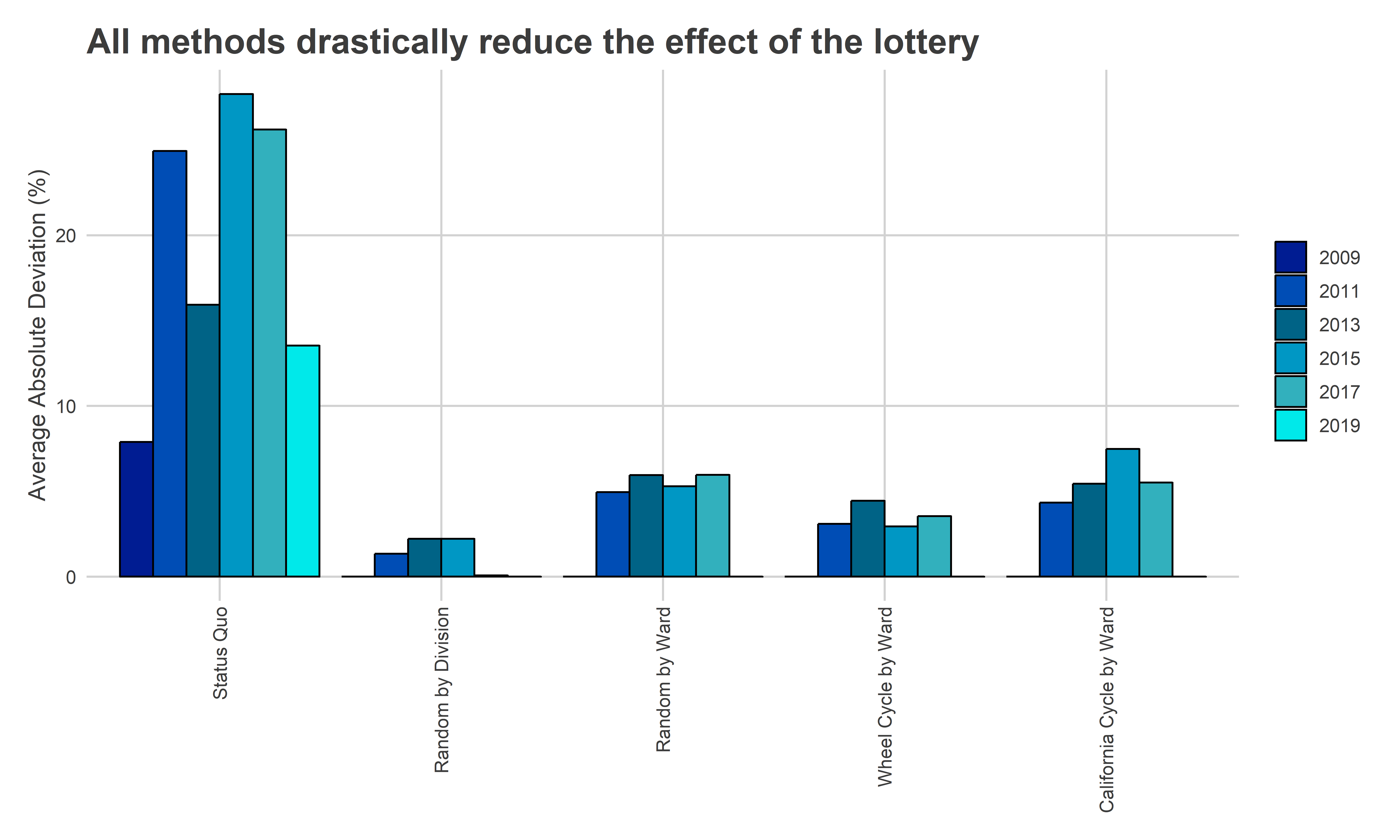
The current system has an average deviation of 19.5%; the randomness of ballot position changes a candidate’s probability of winning by 19.5%, on average. Randomizing by Division lessens that to 1.0% on average; now, the swings due to randomness changes a candidate’s probability of winning by only 1.0%. Randomizing by Ward lessens it to 3.7%, and Cycling by the wheel to 2.3%.
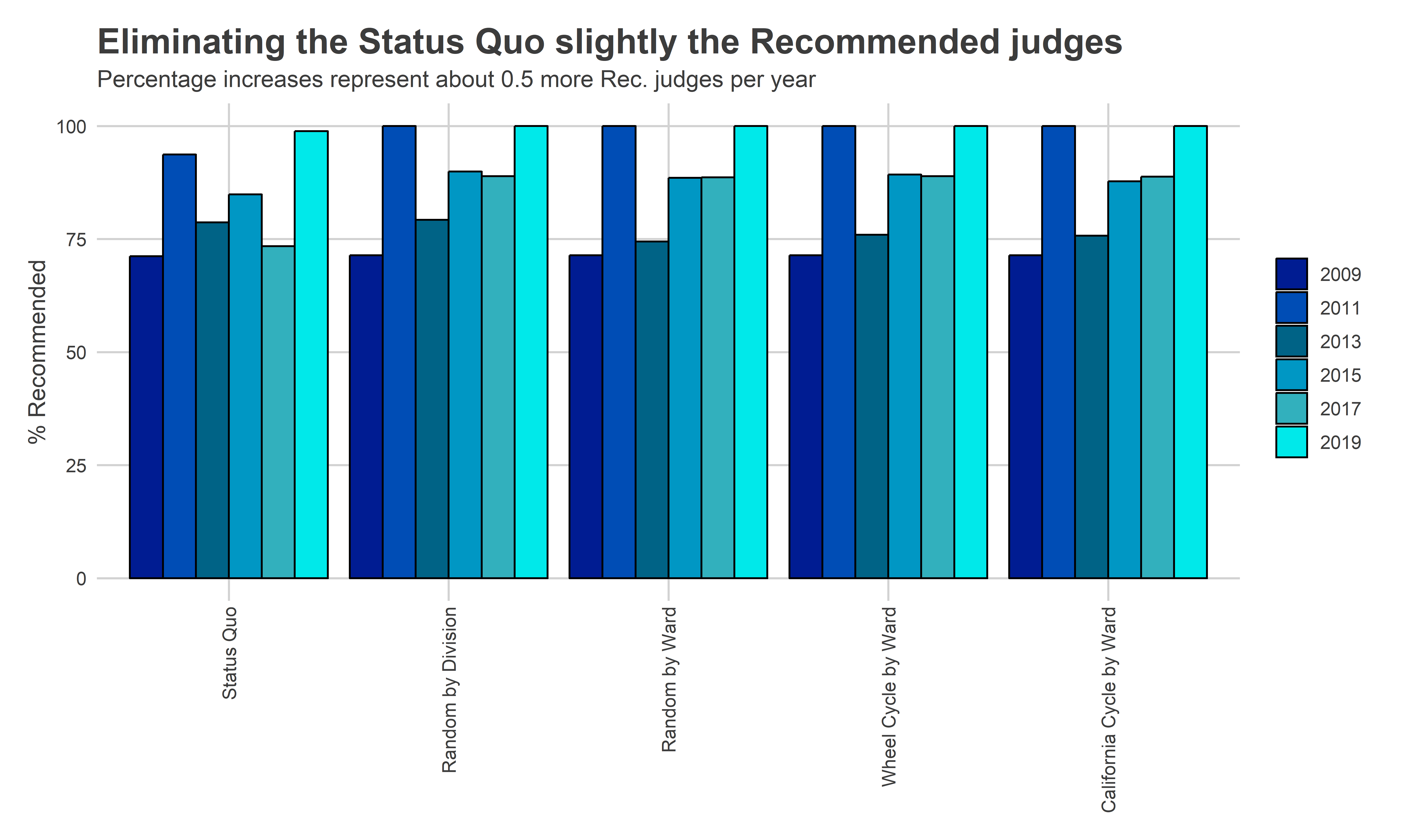
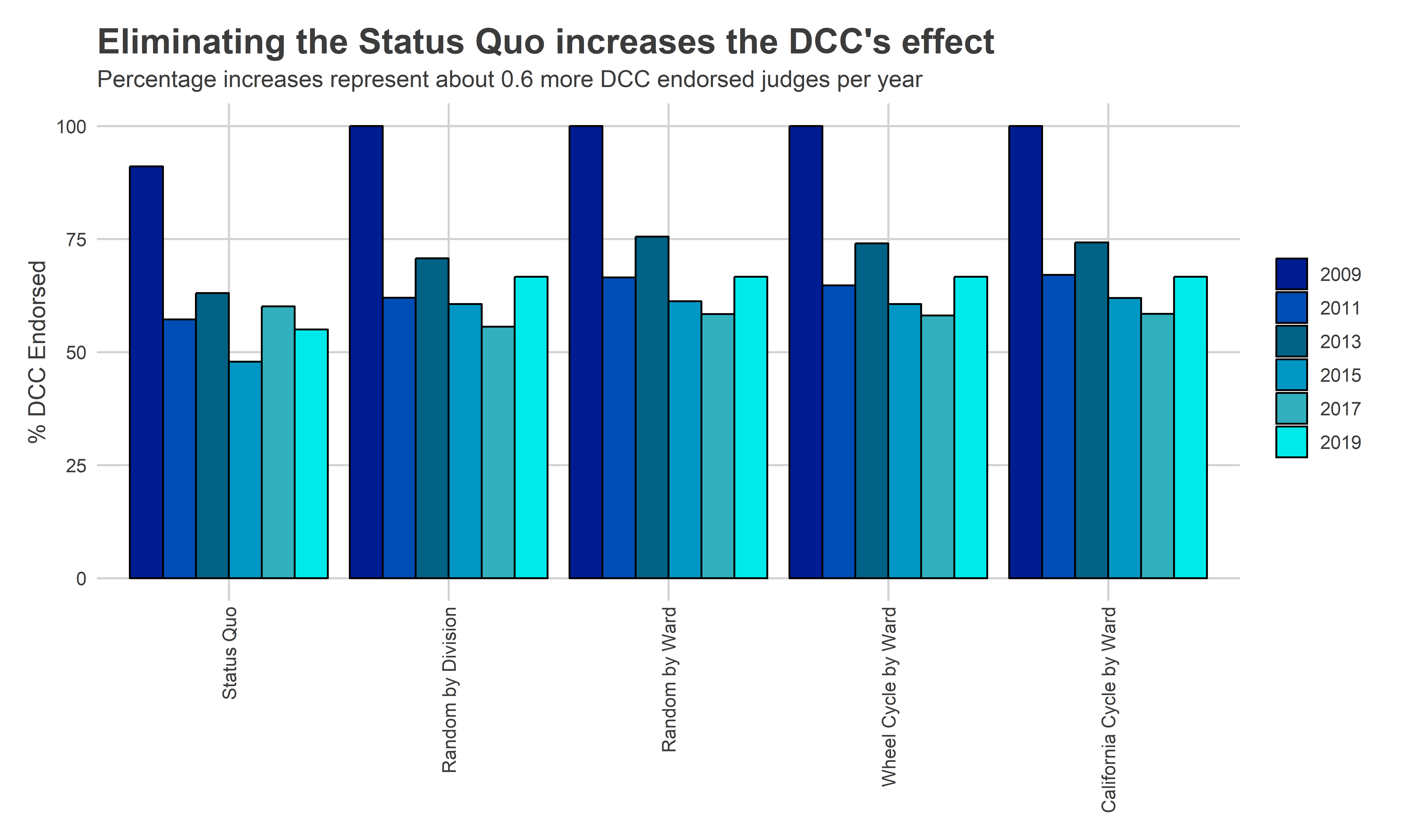
Removing the effect of ballot position makes the other determinants–Bar Recommendations and DCC endorsements–more effective, but less so than I expected. Under the Status Quo, 83% of winners are Recommended by the Bar on average, while 88%, 87%, and 87% are for Division randomization, Ward randomization, and the Wheel, respectively. An average 63% of the winners are endorsed by the DCC under the Status Quo, which becomes 70%, 71%, and 71% under Division randomization, Ward randomization, and the Wheel, respectively.
View code
plot_df <- results_df %>% left_join(
  out_df %>% rename(year=Year, nwin = `Number of\nWinners`) %>%
    select(year, nwin)
) %>%
  mutate(
    `% Recommended` = `Recommended Winners`/nwin * 100,
    `% DCC Endorsed` = `DCC-Endorsed Winners`/nwin * 100
  )

cols <- c(
  "Average Absolute Deviation (%)",
  "% Recommended",
  "% DCC Endorsed"
)

plot_var <- function(var, title = NULL, subtitle=NULL){
  var <- enquo(var)
  ggplot(
    plot_df,
    aes(
      y = !!var,
      x = factor(method, levels = replace_method),
      group=interaction(method, year), fill=as.character(year)
    )
  ) +
    geom_bar(stat="identity", position="dodge", color="black") +
    xlab(NULL) + ylab(rlang::as_name(var)) +
    scale_fill_discrete(
      NULL,
      h = c(253, 253), c = c(50, 100),
      l = seq(10, 80, length.out = 6)
    ) +
    theme_sixtysix() %+replace%
    theme(
      axis.text.x = element_text(angle=90, hjust=1),
      legend.position = "right",
      legend.direction = "vertical"
    ) +
    ggtitle(title, subtitle)
}

plot_var(
  `Average Absolute Deviation (%)`,
  "All methods drastically reduce the effect of the lottery"
)
View code
plot_var(
  `% Recommended`,
  "Eliminating the Status Quo slightly the Recommended judges",
  "Percentage increases represent about 0.5 more Rec. judges per year"
)
View code
plot_var(
  `% DCC Endorsed`,
  "Eliminating the Status Quo increases the DCC's effect",
   "Percentage increases represent about 0.6 more DCC endorsed judges per year"
)
Remember, these estimates assume the same effects as under the current status quo. This includes a world where the DCC and fundraisers take the ballot position into effect. In a new world, where the lottery no longer mattered, the DCC would likely endorse a different set of candidates, and other skills would determine which candidates raised money. Thus, the effects of those traits could in general be different. But they would almost certainly be more determinative of the winners. And we would no longer elect our judges by random lottery.