Could Maria Lose?
Maria Quiñones-Sánchez is facing a significant challenge for the second election in a row. The three term councilmember was challenged by Manny Morales four years ago, and eked out a 53.5% – 46.5% win, a margin of only 868 votes. She’s being challenged again this year by state Rep and ward leader Angel Cruz. What should we expect?
The 7th district is decidedly different from Jannie Blackwell’s 3rd or Kenyatta Johnson’s 2nd. Those heavily-segregated districts had clear racial coalitions that swung differently from year to year.
North Philly’s 7th is segregated, but more homogenously so. It’s Philadelphia’s most Hispanic district, with a predominantly Black section of Frankford in the Northeast and the beginnings of White Kensington gentrification expanding up in the South. In the manner of Philadelphia’s Hispanic neighborhoods, it has very low turnout.
But the vote this May won’t split along racial lines. Instead, what matters is the Wards.
Four years ago, three of the district’s ward leaders coordinated to support Quiñones-Sánchez’s challenger, with heavy involvement from Johnny Doc’s Local 98, including more than $100,000 in contributions and over 1,000 “voter assist requests” for help in the voting booth.
The leaders are coordinating a challenge again, with a candidate Cruz who has apparently less baggage than Morales.
(I can’t quite do justice to the story of this race. Check out the links above and Billy Penn’s summary. )
The challenge seems stronger this year, with eight of the twelve ward leaders in the district supporting Cruz in the party endorsement. But Quiñones-Sánchez held it off last year. What should we expect?
District 7’s voting blocks
The 7th Council district covers North Philly, with 6th and 9th Streets serving as the Western border.
View code
library(tidyverse)
library(rgdal)
library(rgeos)
library(sp)
library(ggmap)

sp_council <- readOGR("../../../data/gis/city_council/Council_Districts_2016.shp", verbose = FALSE)
sp_council <- spChFIDs(sp_council, as.character(sp_council$DISTRICT))

sp_divs <- readOGR("../../../data/gis/2016/2016_Ward_Divisions.shp", verbose = FALSE)
sp_divs <- spChFIDs(sp_divs, as.character(sp_divs$WARD_DIVSN))
sp_divs <- spTransform(sp_divs, CRS(proj4string(sp_council)))

load("../../../data/processed_data/df_major_2017_12_01.Rda")

ggcouncil <- fortify(sp_council) %>% mutate(council_district = id)
ggdivs <- fortify(sp_divs) %>% mutate(WARD_DIVSN = id)
View code
## Need to add District result election from 2015
raw_d2 <-  read.csv("../../../data/raw_election_data/2015_primary.csv")
raw_d2 <- raw_d2 %>%
  filter(OFFICE == "DISTRICT COUNCIL-7TH DISTRICT-DEM") %>%
  mutate(
    WARD = sprintf("%02d", asnum(WARD)),
    DIV = sprintf("%02d", asnum(DIVISION))
  )

load('../../../data/gis_crosswalks/div_crosswalk_2013_to_2016.Rda')
crosswalk_to_16 <- crosswalk_to_16 %>% group_by() %>%
  mutate(
    WARD = sprintf("%02s", as.character(WARD)),
    DIV = sprintf("%02s", as.character(DIV))
  )

d2 <- raw_d2 %>%
  left_join(crosswalk_to_16) %>%
  group_by(WARD16, DIV16, OFFICE, CANDIDATE) %>%
  summarise(VOTES = sum(VOTES * weight_to_16)) %>%
  mutate(PARTY="DEMOCRATIC", year="2015", election="primary")
df_major <- bind_rows(df_major, d2)
View code
races <- tribble(
  ~year, ~OFFICE, ~office_name,
  "2015", "MAYOR", "Mayor",
  "2015", "DISTRICT COUNCIL-7TH DISTRICT-DEM", "Council 7th District",
  "2016", "PRESIDENT OF THE UNITED STATES", "President",
  "2017", "DISTRICT ATTORNEY", "District Attorney"
) %>% mutate(election_name = paste(year, office_name))

candidate_votes <- df_major %>%
  filter(election == "primary" & PARTY == "DEMOCRATIC") %>%
  inner_join(races %>% select(year, OFFICE)) %>%
  mutate(WARD_DIVSN = paste0(WARD16, DIV16)) %>%
  group_by(WARD_DIVSN, OFFICE, year, election) %>%
  mutate(
    total_votes = sum(VOTES),
    pvote = VOTES / sum(VOTES)
  ) %>%
  group_by()

turnout_df <- candidate_votes %>%
  filter(!grepl("COUNCIL", OFFICE)) %>%
  group_by(WARD_DIVSN, OFFICE, year, election) %>%
  summarise(total_votes = sum(VOTES)) %>%
  left_join(
    sp_divs@data %>% select(WARD_DIVSN, AREA_SFT)
  )

turnout_df$AREA_SFT <- asnum(turnout_df$AREA_SFT)
View code
get_labpt_df <- function(sp){
  mat <- sapply(sp@polygons, slot, "labpt")
  df <- data.frame(x = mat[1,], y=mat[2,])
  return(
    cbind(sp@data, df)
  )
}

ggplot(ggcouncil, aes(x=long, y=lat)) +
  geom_polygon(
    aes(group=group),
    fill = strong_green, color = "white", size = 1
  ) +
  geom_text(
    data = get_labpt_df(sp_council),
    aes(x=x,y=y,label=DISTRICT)
  ) +
  theme_map_sixtysix() +
  coord_map() +
  ggtitle("Council Districts")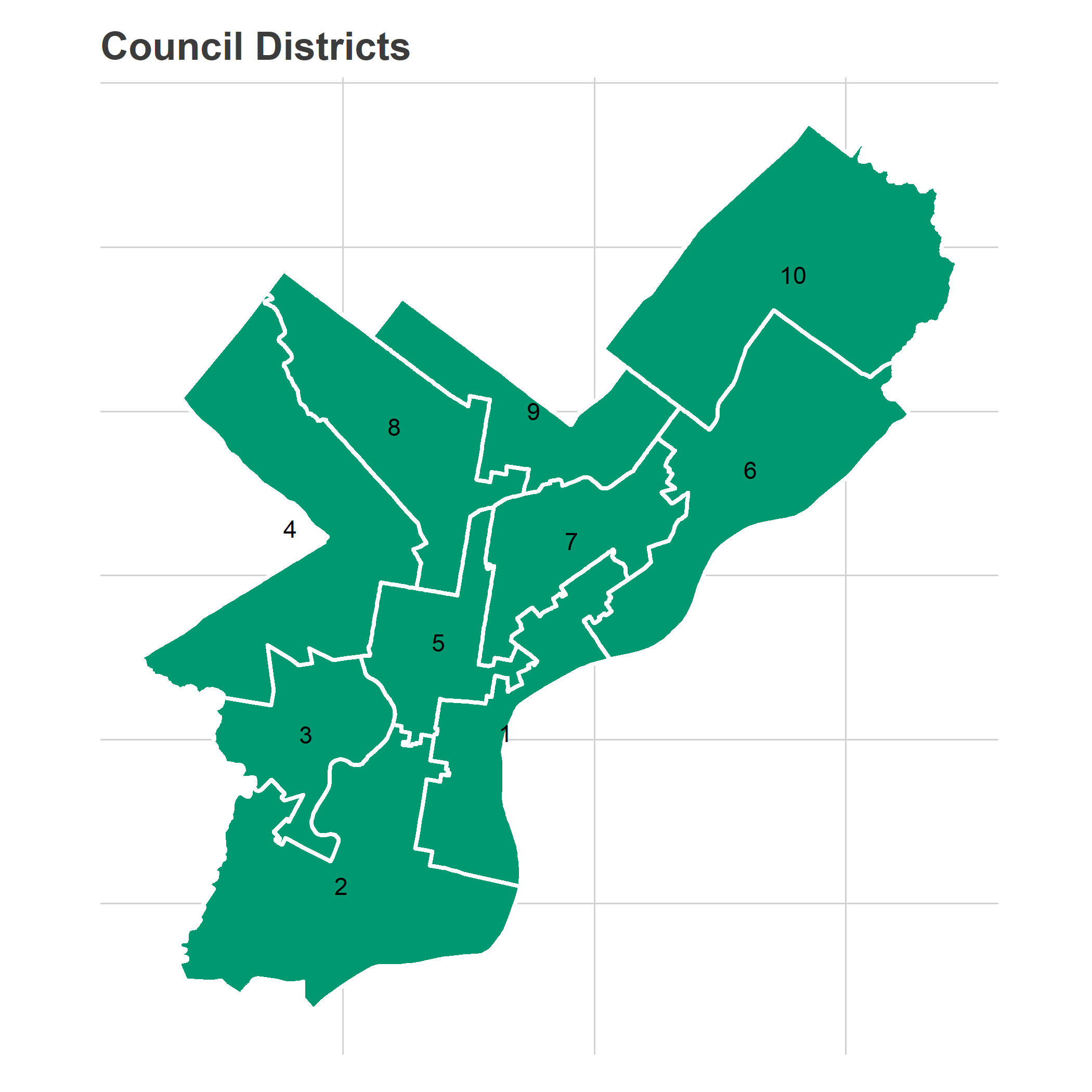
View code
DISTRICT <- "7"
sp_district <- sp_council[row.names(sp_council) == DISTRICT,]
bbox <- sp_district@bbox
## expand the bbox 20%for mapping
bbox <- rowMeans(bbox) + 1.2 * sweep(bbox, 1, rowMeans(bbox))
if(file.exists("map_cache.Rda")){
load("map_cache.Rda")
} else {
basemap <- get_map(bbox, maptype="toner-lite", filename="map_cache.png")
save(basemap, file="map_cache.Rda")
}
district_map <- ggmap(
basemap,
extent="normal",
base_layer=ggplot(ggcouncil, aes(x=long, y=lat, group=group)),
maprange = FALSE
)
## without basemap:
# district_map <- ggplot(ggcouncil, aes(x=long, y=lat, group=group))
district_map <- district_map +
theme_map_sixtysix() +
coord_map(xlim=bbox[1,], ylim=bbox[2,])
sp_divs$council_district <- over(
gCentroid(sp_divs, byid = TRUE),
sp_council
)$DISTRICT
polygon_in_bbox <- function(p) {
coords <- p@Polygons[[1]]@coords
any(
coords[,1] > bbox[1,1] &
coords[,1] < bbox[1,2] &
coords[,2] > bbox[2,1] &
coords[,2] < bbox[2,2]
)
}
sp_divs$in_bbox <- sapply(
sp_divs@polygons,
polygon_in_bbox
)
ggdivs <- ggdivs %>%
left_join(
sp_divs@data %>% select(WARD_DIVSN, in_bbox)
)
district_map +
geom_polygon(
aes(alpha = (id == DISTRICT)),
fill="black",
color = "grey50",
size=2
) +
scale_alpha_manual(values = c(`TRUE` = 0.2, `FALSE` = 0), guide = FALSE) +
ggtitle(sprintf("Council District %s", DISTRICT))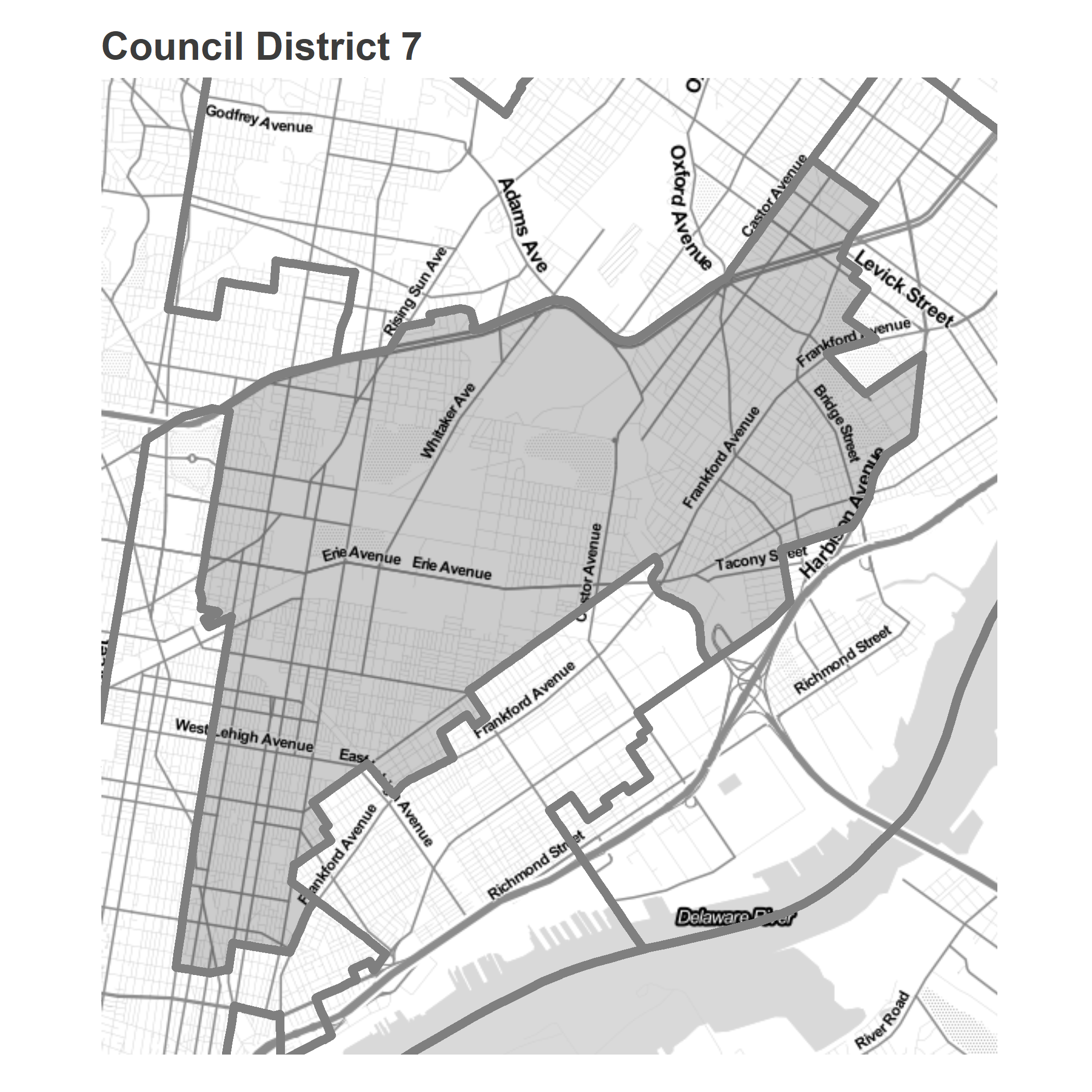 The district has the lowest turnout in the city. Philadelphia’s Hispanic neighborhoods have very low turnout, and this district is the most Hispanic. Curiously, not only does the neighborhood have low turnout in Presidential elections, but it then has disproportionately lower turnout in municipal elections even given that: even residents who vote for President are less likely to vote in other years.
View code
# hist(turnout_df$total_votes / turnout_df$AREA_SFT, breaks = 1000)
turnout_df <- turnout_df %>%
left_join(races)
district_map +
geom_polygon(
data = ggdivs %>%
filter(in_bbox) %>%
left_join(turnout_df, by =c("id" = "WARD_DIVSN")),
aes(fill = pmin(total_votes / AREA_SFT, 0.0005) * 5280^2)
) +
scale_fill_viridis_c(
"Votes per mile",
labels=scales::comma,
guide=guide_colorbar(label.theme=element_text(angle=90, size = 10), label.hjust=1)
) +
geom_polygon(
fill=NA,
color = "white",
size=1
) +
facet_wrap(~ election_name) +
expand_limits(fill=0) +
ggtitle(
"Votes per mile in the Democratic Primary",
sprintf("Council District %s", DISTRICT)
) +
theme(legend.position = "bottom", legend.direction = "horizontal")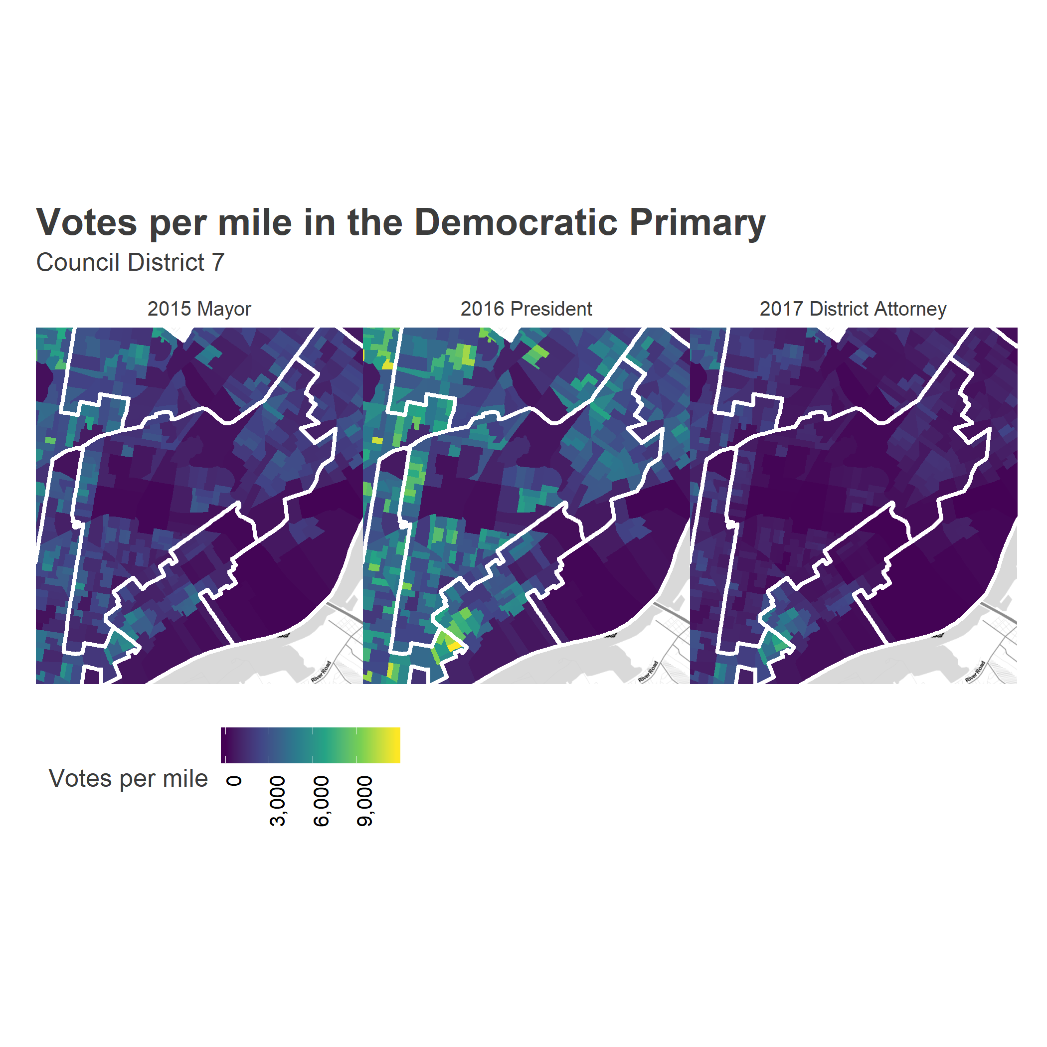 The district as a whole cast 25,000 votes in the 2016 Presidential primary, 12,000 last time Quninones-Sanchez ran, and only 6,000 in the the 2017 District Attorney race. They did not see the Krasner surge.
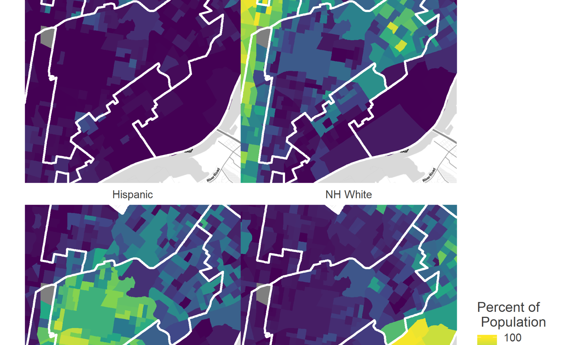
Demographically, the district is Philadelphia’s most heavily hispanic, though with Frankford in its Northeast being predominantly Black:
View code
bg_17_acs <- read.csv("../../../data/census/acs_2013_2017_phila_bg_race_income.csv")
bg_17_acs <- bg_17_acs %>%
  mutate(Geo_FIPS = as.character(Geo_FIPS)) %>%
  select(Geo_FIPS, pop, pop_nh_white, pop_nh_black, pop_nh_asian, pop_hisp, pop_median_income_2017)

library(tigris)
options(tigris_use_cache = TRUE)
bg_shp <- block_groups(42, 101, year = 2015)
bg_shp <- spChFIDs(bg_shp, as.character(bg_shp$GEOID))
bg_shp <- spTransform(bg_shp, CRS(proj4string(sp_divs)))

bg_shp$in_bbox <- sapply(
  bg_shp@polygons,
  polygon_in_bbox
)

gg_bgs <- fortify(bg_shp)
gg_bgs <- gg_bgs %>%
  left_join(bg_shp@data[,c("GEOID", "ALAND", "in_bbox")], by = c("id" = "GEOID")) %>%
  left_join(bg_17_acs, by = c("id" = "Geo_FIPS"))

district_map +
  geom_polygon(
    data = gg_bgs %>%
      filter(in_bbox) %>%
      gather("key", "race_pop",pop_nh_white, pop_nh_black, pop_nh_asian, pop_hisp) %>%
      mutate(
        pct_pop = 100 * race_pop / pop,
        race = c(
          pop_hisp = "Hispanic", pop_nh_white="NH White", pop_nh_black="Black", pop_nh_asian="Asian"
        )[key]
      ),
    aes(fill = pct_pop)
  ) +
  geom_polygon(
    fill=NA,
    color = "white",
    size=1
  ) +
  facet_wrap(~race) +
  scale_fill_viridis_c("Percent of\n Population") +
  theme(legend.position = "right") +
  ggtitle(sprintf("Race and Ethnicity of District %s", DISTRICT))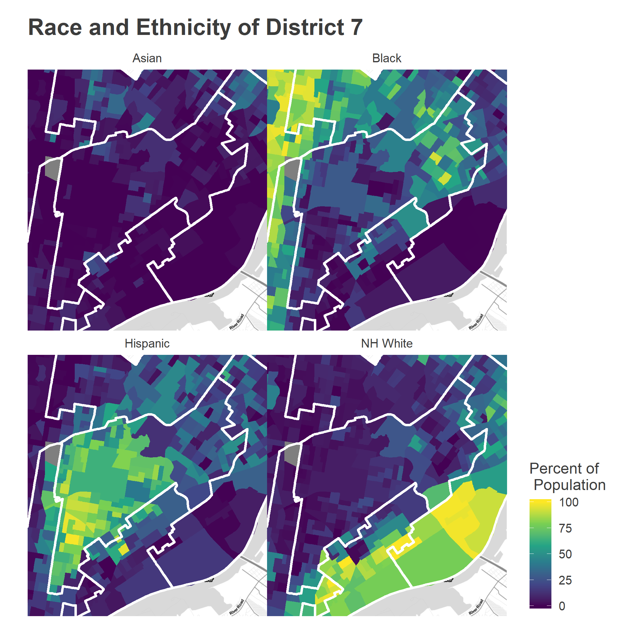
The district is less obviously politically split than other parts of the city. When it does split, it often does so for Latino candidates. Below are the results from the last race for the 7th and three other recent, compelling Democratic Primary races: 2015 Mayor, 2016 President, and 2017 District Attorney. The maps below show the vote for the top two candidates in District 2 (except for City Council in 2015, where I use Helen Gym and Isaiah Thomas, who were 4th and 5th in the district, and 5th and 6th citywide.)
View code
candidate_votes <- candidate_votes %>%
left_join(sp_divs@data %>% select(WARD_DIVSN, council_district))
## Choose the top two candidates in district 3
## Except for city council, where we choose Gym and Thomas
# candidate_votes %>%
# group_by(OFFICE, year, CANDIDATE) %>%
# summarise(
# city_votes = sum(VOTES),
# district_votes = sum(VOTES * (council_district == DISTRICT))
# ) %>%
# arrange(desc(city_votes)) %>%
# filter(OFFICE == "MAYOR")
candidates_to_compare <- tribble(
~year, ~OFFICE, ~CANDIDATE, ~candidate_name, ~row,
"2015", "DISTRICT COUNCIL-7TH DISTRICT-DEM", "MANNY MORALES", "Manny Morales", 1,
"2015", "DISTRICT COUNCIL-7TH DISTRICT-DEM", "MARIA QUINONES SANCHEZ", "Maria Quiñones-Sánchez", 2,
"2015", "MAYOR", "JIM KENNEY", "Jim Kenney", 2,
"2015", "MAYOR", "NELSON DIAZ", "Nelson Diaz", 1,
"2016", "PRESIDENT OF THE UNITED STATES", "BERNIE SANDERS", "Bernie Sanders", 2,
"2016", "PRESIDENT OF THE UNITED STATES", "HILLARY CLINTON", "Hillary Clinton", 1,
"2017", "DISTRICT ATTORNEY", "LAWRENCE S KRASNER", "Larry Krasner", 2,
"2017", "DISTRICT ATTORNEY", "RICH NEGRIN","Rich Negrin", 1
)
candidate_votes <- candidate_votes %>%
left_join(races) %>%
left_join(candidates_to_compare)
vote_adjustment <- function(pct_vote, office){
ifelse(office == "COUNCIL AT LARGE", pct_vote * 4, pct_vote)
}
district_map +
geom_polygon(
data = ggdivs %>%
filter(in_bbox) %>%
left_join(
candidate_votes %>% filter(!is.na(row))
),
aes(fill = 100 * vote_adjustment(pvote, OFFICE))
) +
scale_fill_viridis_c("Percent of Vote") +
theme(
legend.position = "bottom",
legend.direction = "horizontal",
legend.justification = "center"
) +
geom_polygon(
fill=NA,
color = "white",
size=1
) +
geom_label(
data=candidates_to_compare %>% left_join(races),
aes(label = candidate_name),
group=NA,
hjust=0, vjust=1,
x=bbox[1,1],
y=bbox[2,2]
) +
facet_grid(row ~ election_name) +
theme(strip.text.y = element_blank()) +
ggtitle(
sprintf("Candidate performance in District %s", DISTRICT)
# "Percent of vote (times 4 for Council, times 1 for other offices)"
)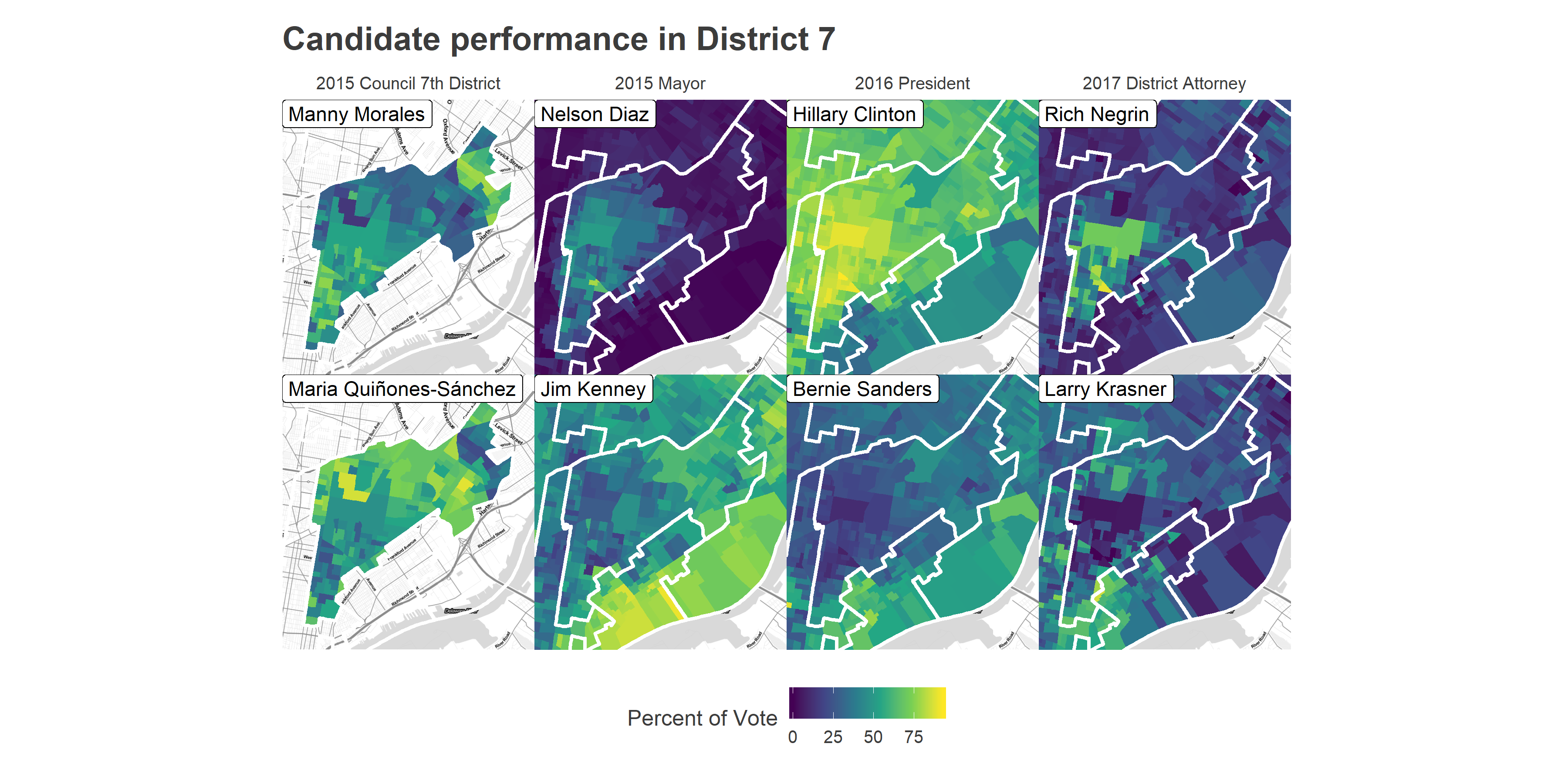 The district split for Mayor and for District Attorney along racial lines: the densest latino neighborhoods voted for Diaz and Negrin, while the rest of the district voted for the citywide winners Kenney and Krasner. However, the cleavage was geographically different for Quiñones-Sánchez v Morales, presumably because both candidates were latinx. That’s true this time around, too.
Just because there wasn’t a racial split doesn’t mean the district voted uniformly. There indeed were stark variations in how Quiñones-Sánchez did, but the reason isn’t obviously clear. She did well in the Northwest of the district, especially West of 6th St, and in the Northeast of the district except for South of the Boolevard and East of Oxford.
What gives? Those are all Ward boundaries.
View code
wards <- readOGR("../../../data/gis/2016","2016_Wards", verbose=FALSE) %>%
  spTransform(CRS(proj4string(sp_divs)))

ggwards <- fortify(wards)

wards_centers <- sapply(wards@polygons, slot, "labpt") %>% t
wards_centers <- as.data.frame(wards_centers)
names(wards_centers) <- c("x", "y")

wards@data <- cbind(wards@data, wards_centers)


district_map +
  geom_polygon(data = ggwards, fill = NA, color = strong_red, size= 2) +
  geom_polygon(
    data = ggcouncil %>% filter(council_district == 7),
    fill=NA,
    color = "black",
    size = 2
  ) +
  geom_text(
    data = wards@data,
    aes(x=x, y=y, label=WARD),
    group = NA,
    color = strong_red,
    fontface="bold"
  ) +
  ggtitle("The wards of District 7")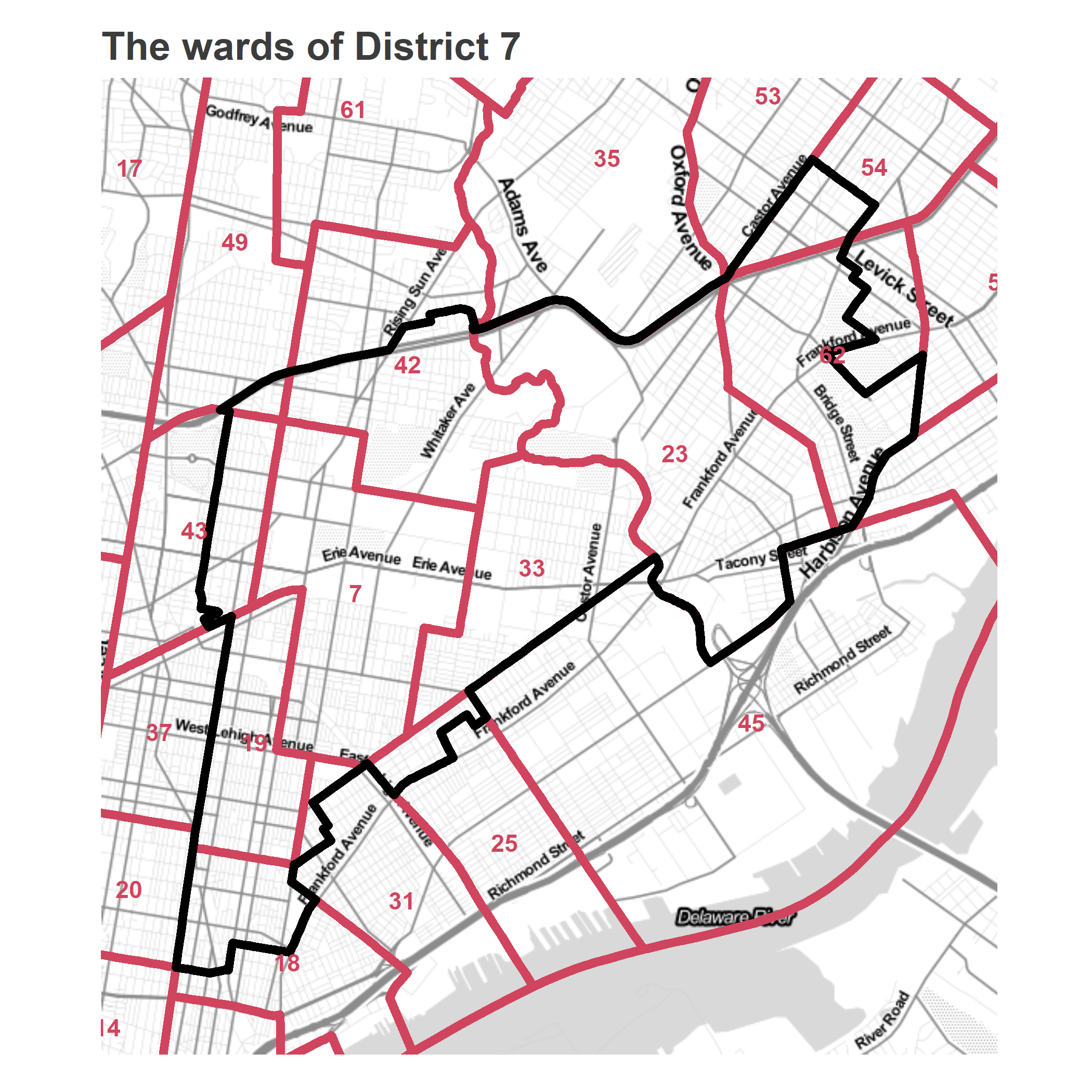
Quiñones-Sánchez’s performance is a potent example of the power of Ward endorsements: she performed very differently in different wards, in some cases on literally the other side of the street. That thin sliver in the Northwest of the District where she did exceptionally well was the 43rd Ward. She received large percentages in the 23rd and 54th in the Northwest, too, but that region where she did poorly, South of the Boolevard and East of Oxford, exactly lines up with the boundaries to the 62nd.
So the question for the 2019 race becomes how the ward endorsements will shake out and how powerful each ward is, both in terms of ability to swing the vote and typicaly turnout. Below are measures of their strength. I’ve also pulled in the Ward leaders’ endorsements from the DCC vote.
View code
## Get vote-weighted populations
div_centroids <- gCentroid(sp_divs[sp_divs$council_district == DISTRICT,], byid=TRUE)
div_centroids$WARD_DIVSN <- attr(div_centroids@coords, "dimnames")[[1]]
div_centroids$bg_GEOID <- over(div_centroids, bg_shp)$GEOID
div_centroids@data <- left_join(div_centroids@data, bg_17_acs, by = c("bg_GEOID" = "Geo_FIPS"))

district_7_results <- df_major %>%
  filter(
    year == 2015 & grepl("7TH DISTRICT", OFFICE) & CANDIDATE != "Write In"
  ) %>%
  mutate(WARD_DIVSN = paste0(WARD16, DIV16)) %>%
  select(WARD_DIVSN, CANDIDATE, VOTES) %>%
  spread(CANDIDATE, VOTES) %>%
  mutate(
    total_votes = (`MARIA QUINONES SANCHEZ` + `MANNY MORALES`),
    p_quinones_sanchez = `MARIA QUINONES SANCHEZ` / total_votes
  )

div_centroids@data <- left_join(div_centroids@data, district_7_results)

ward_pops <- div_centroids@data %>%
  mutate(ward = substr(WARD_DIVSN, 1, 2)) %>%
  group_by(ward) %>%
  summarise(
    p_quinones_sanchez = 100 * weighted.mean(p_quinones_sanchez, w = total_votes),
    pct_nh_white = 100 * weighted.mean(pop_nh_white / pop, w = total_votes),
    pct_nh_black = 100 * weighted.mean(pop_nh_black / pop, w = total_votes),
    pct_nh_asian = 100 * weighted.mean(pop_nh_asian / pop, w = total_votes),
    pct_hisp = 100 * weighted.mean(pop_hisp / pop, w = total_votes),
    council_votes = sum(total_votes)
  )

ward_results <- df_major %>%
  mutate(WARD_DIVSN = paste0(WARD16, DIV16)) %>%
  inner_join(
    tribble(
      ~year, ~election, ~PARTY, ~OFFICE,
      "2016", "primary", "DEMOCRATIC", "PRESIDENT OF THE UNITED STATES",
      "2017", "primary", "DEMOCRATIC", "DISTRICT ATTORNEY"
    )
  ) %>%
  inner_join(div_centroids@data) %>%
  group_by(year, WARD16) %>%
  summarise(total_votes = sum(VOTES)) %>%
  group_by() %>%
  group_by(year) %>%
  mutate(pct_of_year = 100 * total_votes / sum(total_votes)) %>%
  gather("key", "value", total_votes, pct_of_year) %>%
  unite("key", key, year) %>%
  spread(key, value)

ward_pops <- ward_pops %>%
  left_join(
    ward_results %>% rename(ward = WARD16)
  ) %>%
  group_by() %>%
  mutate(pct_of_year_2015 = 100 * council_votes / sum(council_votes))

ward_leaders <- tribble(
  ~ward, ~leader, ~endorsement,
  "07", "Angel Cruz", "Cruz",
  "18", "Theresa Alicea", "Cruz",
  "19", "Carlos Matos","Cruz",
  "23", "Timothy Savage","Quiñones-Sánchez",
  "25", "Thomas Johnson","Cruz",
  "31", "Margaret Rzepski","Cruz",
  "33", "Donna Aument","Cruz",
  "42", "Sharon Vaughn","Quiñones-Sánchez",
  "43", "Emilio Vazquez","Quiñones-Sánchez",
  "49", "Shirley Gregory","Cruz",
  "54", "Alan Butkovitz","Quiñones-Sánchez",
  "62", "Margaret Tartaglione","Cruz"
)

ward_pops <- ward_pops %>% left_join(ward_leaders)

knitr::kable(
  ward_pops %>%
    select(ward, council_votes, pct_of_year_2015, p_quinones_sanchez, leader, endorsement, pct_hisp, pct_nh_white, pct_nh_black, total_votes_2016, pct_of_year_2016, total_votes_2017, pct_of_year_2017) %>%
    arrange(desc(council_votes)),
    digits=0,
    format.args=list(big.mark=','),
    col.names=c("Ward", "Votes for the 7th in 2015 Primary", "Pct of District", "% for Quiñones-Sánchez",  "Leader", "Endorsement", "% Hispanic", "% White", "% Black", "Votes in 2016 Primary", "Pct of District", "Votes in 2017 Primary", "Pct of District")
)| Ward | Votes for the 7th in 2015 Primary | Pct of District | % for Quiñones-Sánchez | Leader | Endorsement | % Hispanic | % White | % Black | Votes in 2016 Primary | Pct of District | Votes in 2017 Primary | Pct of District |
|---|---|---|---|---|---|---|---|---|---|---|---|---|
| 23 | 2,108 | 17 | 71 | Timothy Savage | Quiñones-Sánchez | 28 | 19 | 46 | 4,021 | 16 | 1,284 | 22 |
| 62 | 1,774 | 14 | 33 | Margaret Tartaglione | Cruz | 31 | 22 | 41 | 3,546 | 14 | 913 | 16 |
| 19 | 1,683 | 14 | 37 | Carlos Matos | Cruz | 77 | 6 | 15 | 2,817 | 11 | 589 | 10 |
| 07 | 1,655 | 14 | 49 | Angel Cruz | Cruz | 80 | 8 | 11 | 3,340 | 13 | 549 | 9 |
| 33 | 1,455 | 12 | 57 | Donna Aument | Cruz | 63 | 10 | 18 | 3,337 | 13 | 566 | 10 |
| 42 | 1,177 | 10 | 63 | Sharon Vaughn | Quiñones-Sánchez | 64 | 8 | 16 | 2,581 | 10 | 543 | 9 |
| 43 | 1,124 | 9 | 65 | Emilio Vazquez | Quiñones-Sánchez | 66 | 3 | 29 | 2,259 | 9 | 445 | 8 |
| 18 | 611 | 5 | 51 | Theresa Alicea | Cruz | 45 | 29 | 16 | 1,340 | 5 | 527 | 9 |
| 54 | 311 | 3 | 66 | Alan Butkovitz | Quiñones-Sánchez | 17 | 18 | 49 | 906 | 4 | 196 | 3 |
| 25 | 133 | 1 | 59 | Thomas Johnson | Cruz | 47 | 33 | 15 | 350 | 1 | 77 | 1 |
| 49 | 117 | 1 | 72 | Shirley Gregory | Cruz | 28 | 0 | 72 | 192 | 1 | 44 | 1 |
| 31 | 98 | 1 | 63 | Margaret Rzepski | Cruz | 23 | 57 | 8 | 265 | 1 | 129 | 2 |
The ward with the most votes for the 7th in 2015 also voted hard for Quiñones-Sánchez: the 23rd. Her 71% dominance of the 2,108 votes cast gave her an 886 vote edge, more than what she won the entire District by. That ward, which includes the district’s predominantly Black neighborhoods, turns out stronger than the rest. It represented 17% of the district’s votes in 2015, and then a whopping 22% of the votes in low-turnout 2017.
The next three most dominant wards were 62, 19, and 7 and those went for Morales with 63, 67, and 51% of the vote. (Notice that 62 is actually split by Council Districts; the number above is only for District 7). Those are the three wards led by State Senator Margaret Tartaglione, Carlos Matos, and Angel Cruz himself, the ward leaders that organized the challenge. Quiñones-Sánchez won all of the other Wards, but those three were enough to make the race close.
We can simplify the table above by combining all of the wards whose leaders supported Quiñones-Sánchez and those whose leaders supported Cruz.
View code
get_line <- function(x_total_votes, y_total_votes){
  ## solve p_x t_x+ p_y t_y > 50
  tot <- x_total_votes + y_total_votes
  tx <- x_total_votes / tot
  ty <- y_total_votes / tot

  slope <- -tx / ty
  intercept <- 50 / ty  # use 50 since proportions are x100
  c(intercept, slope)
}

endorsement_summary <- ward_pops %>%
  group_by(endorsement) %>%
  summarise(
    p_quinones_sanchez = weighted.mean(p_quinones_sanchez, w = council_votes),
    council_votes = sum(council_votes),
    total_votes_2016 = sum(total_votes_2016),
    total_votes_2017 = sum(total_votes_2017)
  )

candidate_results = with(
  endorsement_summary,
  tribble(
    ~candidate,
    ~p_in_mqs_wards,
    ~p_in_challenger_wards,
    ~total_votes_in_mqs_wards,
    ~total_votes_in_challenger_wards,
    "Quiñones-Sánchez",
    p_quinones_sanchez[endorsement == "Quiñones-Sánchez"],
    p_quinones_sanchez[endorsement == "Cruz"],
    council_votes[endorsement == "Quiñones-Sánchez"],
    council_votes[endorsement == "Cruz"],
    "Morales",
    100 - p_quinones_sanchez[endorsement == "Quiñones-Sánchez"],
    100 - p_quinones_sanchez[endorsement == "Cruz"],
    council_votes[endorsement == "Quiñones-Sánchez"],
    council_votes[endorsement == "Cruz"]
  )
) %>%
  mutate(
    votes_in_mqs_wards = p_in_mqs_wards * total_votes_in_mqs_wards / 100,
    votes_in_challenger_wards = p_in_challenger_wards * total_votes_in_challenger_wards / 100
  )

knitr::kable(
  candidate_results %>% select(
    candidate,
    p_in_mqs_wards,
    votes_in_mqs_wards,
    p_in_challenger_wards,
    votes_in_challenger_wards
  ),
  digits=0,
  format.args=list(big.mark=','),
  col.names=c("Candidate", "Percent in MQS-Endorsed Wards", "Votes in MQS-Endorsed Wards", "Percent in Cruz-Endorsed Wards",  "Votes in Cruz-Endorsed Wards")
)| Candidate | Percent in MQS-Endorsed Wards | Votes in MQS-Endorsed Wards | Percent in Cruz-Endorsed Wards | Votes in Cruz-Endorsed Wards |
|---|---|---|---|---|
| Quiñones-Sánchez | 67 | 3,174 | 45 | 3,383 |
| Morales | 33 | 1,546 | 55 | 4,143 |
The four wards that backed Quiñones-Sánchez constituted only 39% of the votes in 2015, but she won them 2:1. The other eight wards combined for 61% of the vote, but Morales only won them 5:4. Quiñones-Sánchez’s wards represented more of the votes in 2017, boding well for this year, but it’s also likely that Cruz will do better in his wards than Morales did.
View code
line_2017 <- with(
  endorsement_summary,
  get_line(
    total_votes_2017[endorsement == "Quiñones-Sánchez"],
    total_votes_2017[endorsement == "Cruz"]
  )
)

line_2015 <- with(
  endorsement_summary,
  get_line(
    council_votes[endorsement == "Quiñones-Sánchez"],
    council_votes[endorsement == "Cruz"]
  )
)

library(ggrepel)
ggplot(
  candidate_results,
  aes(
    x=p_in_mqs_wards,
    y=p_in_challenger_wards
  )
) +
  geom_point() +
  geom_text_repel(aes(label=candidate)) +
  geom_abline(
    intercept = c(line_2015[1], line_2017[1]),
    slope = c(line_2015[2], line_2017[2]),
    linetype="dashed"
  ) +
  coord_fixed() +
  scale_x_continuous(
    "Percent in wards that endorsed Quiñones-Sánchez",
    breaks = seq(0,100,10)
  ) +
  scale_y_continuous(
    "Percent in wards that endorsed Cruz",
    breaks = seq(0, 100, 10)
  ) +
  annotate(
    geom="text",
    label=paste(c(2015, 2017), "turnout"),
    x=c(10, 8),
    y=c(
      line_2015[1] + 10 * line_2015[2],
      line_2017[1] + 8 * line_2017[2]
    ),
    hjust=0,
    vjust=-0.2,
    angle = atan(c(line_2015[2], line_2017[2])) / pi * 180,
    color="grey40"
  )+
  annotate(
    geom="text",
    x = 80,
    y=75,
    label="Candidate wins",
    fontface="bold",
    color = strong_green
  ) +
  geom_hline(yintercept = 50, color="grey50") +
  geom_vline(xintercept = 50, color="grey50")+
  expand_limits(x=100, y=30)+
  theme_sixtysix() +
  ggtitle(
    "The strength of District 7's wards in 2015",
    "Candidates to the top-right of dashed lines win."
  )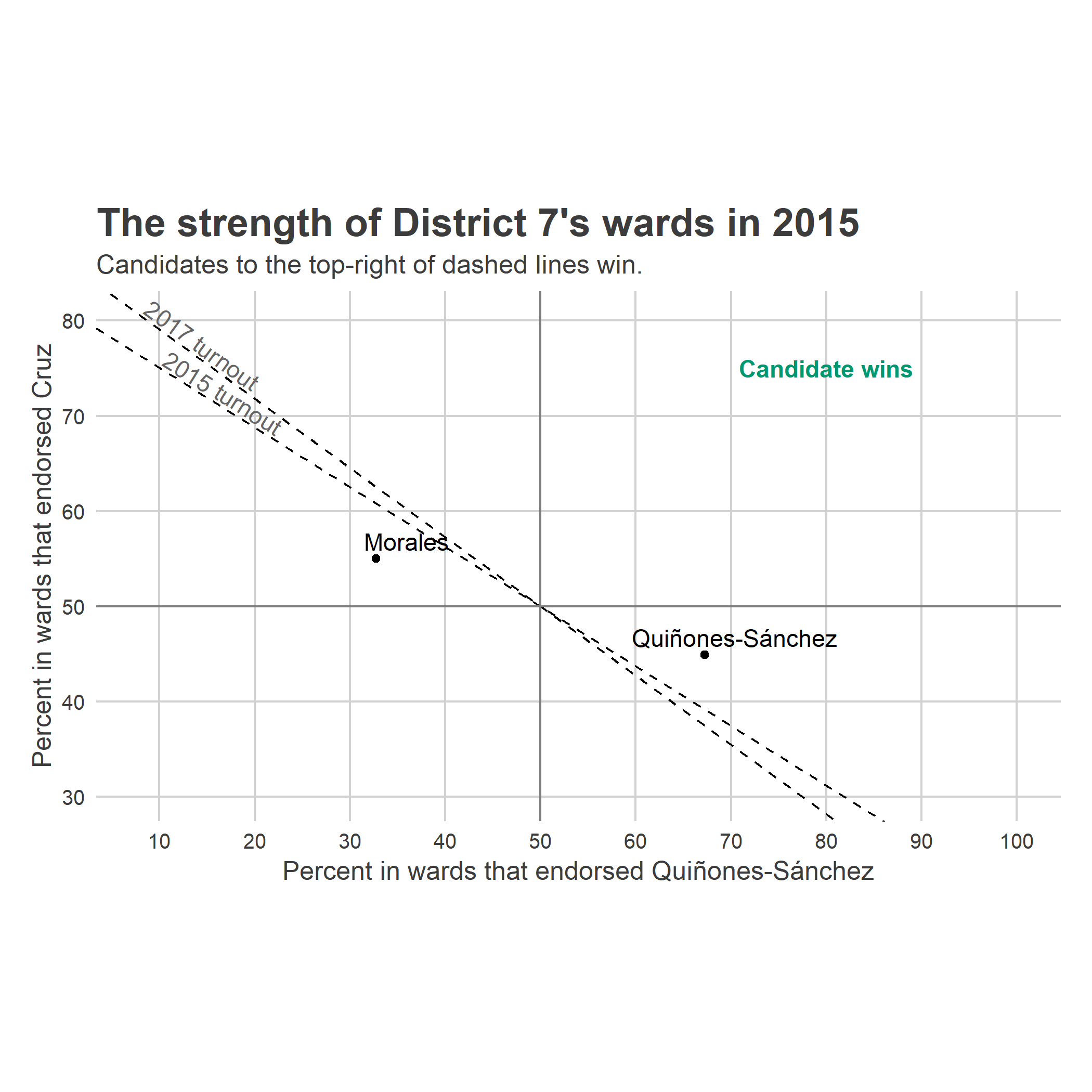
Looking to May
So what are we to make of this race? Keep your eyes on the mobilization behind the Ward endorsements, especially the top turnout wards. Cruz will presumably do even better in his own ward than Morales did, so Quiñones-Sánchez’s success will likely hinge on continued high turnout in the 23rd and trying to consolidate the votes of the rest.
She managed to do that just well enough four years ago to eke out a 9 point victory. This year she faces a candidate without homophobic Facebook posts who also happens to be a Ward leader. If the results in every district were the same as in 2015 except Angel Cruz managed to win 77% of the vote in his own ward, the race would be an exact tie.
It’ll be close.