I’ve been stumped by one thing in the months since the Municipal Primary. My high-level story of Council At Large and Commissioner was the dominance of the Party-backed candidates, and the traditional voting strongholds of Philadelphia’s Black and White Moderate neighborhoods. But the story of Common Pleas was the sweep of Bar-endorsees, typically the darling of the Wealthy Progressives, including Tiffany Palmer, a Highly Recommended candidate who won entirely on the back of Center City and the wealthy Northwest.
How can these two exactly opposite stories emerge in the same election? Is one of them wrong? Let’s dig in.
Who won where
First, some maps.
View code
library(tidyverse)
df_all <- safe_load("../../data/processed_data/df_all_2019_07_09.Rda")

df <- df_all %>%
  mutate(
    OFFICE = ifelse(OFFICE == "COUNCIL AT LARGE", "COUNCIL AT-LARGE", OFFICE)
  ) %>%
  filter(election == "primary" & PARTY == "DEMOCRATIC") %>%
  rename(warddiv=warddiv19, WARD=WARD19, DIV=DIV19) %>%
  group_by(year, OFFICE, CANDIDATE, PARTY, warddiv, WARD, DIV) %>%
  summarise(votes = sum(VOTES))

office_df <- tribble(
  ~office_raw, ~office, ~nwinners,
  "MAYOR", "Mayor", 1,
  "COUNCIL AT-LARGE", "Council At Large", 5,
  "JUDGE OF THE COURT OF COMMON PLEAS", "Common Pleas", 6,
  "CITY COMMISSIONERS", "Commissioner", 2
) %>%
  mutate(office = factor(office, levels=office))

df <- df %>% inner_join(office_df, by = c("OFFICE" = "office_raw"))

##########
## MAPS
##########

# library(leaflet)
# library(leafsync)
library(sf)

divs <- st_read("../../data/gis/2019/Political_Divisions.shp")  %>%
  rename(warddiv=DIVISION_N)wards <- st_read("../../data/gis/2019/Political_Wards.shp") %>%
  mutate(ward = sprintf("%02d", asnum(WARD_NUM)))df <- df %>%
  group_by(year, warddiv, OFFICE, PARTY) %>%
  mutate(
    div_votes = sum(votes),
    pvote = votes / div_votes
  ) %>% group_by()

df_ward <- df %>%
  group_by(year, WARD, OFFICE, CANDIDATE, PARTY) %>%
  summarise(votes = sum(votes)) %>%
  group_by(year, WARD, OFFICE, PARTY) %>%
  mutate(
    div_votes = sum(votes),
    pvote = votes / div_votes
  )


phila_bbox <- st_bbox(divs)

# phila_leaflet <- leaflet() %>%
#   addProviderTiles(providers$Stamen.TonerLite) %>%
#   setView(
#     lng=mean(phila_bbox[c("xmin", "xmax")]),
#     lat=mean(phila_bbox[c("ymin", "ymax")]),
#     zoom = 10
#   )
#
# add_geom <- function(map, geom, value, pal, text=NA){
#   return(
#     map %>% addPolygons(
#       data = geom,
#       weight = 0, color = "white", opacity = 1,
#       fillOpacity = 0.8,  smoothFactor = 0.0,
#       popup = text,
#       fillColor = pal(value)
#     )
#   )
# }
#
# map_candidate <- function(
#   cand_regex,
#   yr,
#   colname="pvote",
#   pal=NULL,
#   use_divs=FALSE,
#   max_value=1.0
# ){
#   if(use_divs){
#     candidate_df <- divs %>%
#       left_join(
#         df %>%
#           filter(year == yr, grepl(cand_regex, CANDIDATE)),
#         by=c("warddiv")
#       ) %>%
#       mutate(
#         geo_name = paste0(
#           "Division ",
#           substr(warddiv, 1, 2), "-", substr(warddiv, 3, 4)
#         )
#       )
#   } else {
#     candidate_df <- wards %>%
#       left_join(
#         df_ward %>%
#           filter(year == yr, grepl(cand_regex, CANDIDATE)),
#         by=c("ward"="WARD")
#       ) %>%
#       mutate(geo_name = paste("Ward", ward))
#   }
#
#   candidate_name <- unique(candidate_df$CANDIDATE)
#
#   if(is.null(pal)) {
#     pal <- colorNumeric("viridis", domain=c(0, max(candidate_df[[colname]])))
#   }
#
#   text <-  with(
#       candidate_df,
#       paste0(
#         geo_name, "<br>",
#         format_name(CANDIDATE), "<br>",
#         scales::comma(votes), " vote", ifelse(votes == 1, "", "s"),
#         " (", round(100*pvote),"%)")
#     )
#
#   phila_leaflet %>% add_geom(
#     candidate_df$geometry,
#     pmin(candidate_df[[colname]], max_value),
#     pal=pal,
#     text=text
#   ) %>% addControl(format_name(candidate_name), position = "topright")
# }
#
# map_candidates <- function(cand_regexes, yr, use_divs=FALSE, max_value=NA, ...){
#   all_regex <- paste0("(",cand_regexes,")", collapse = "|")
#
#   if(is.na(max_value)){
#     if(use_divs) {
#       max_value <- df %>%
#         filter(year == yr, grepl(all_regex, CANDIDATE)) %>%
#         with(max(pvote))
#     } else {
#       max_value <- df_ward %>%
#         filter(year == yr, grepl(all_regex, CANDIDATE)) %>%
#         with(max(pvote))
#     }
#   }
#
#   pal <- colorNumeric("viridis", domain=c(0, max_value))
#   all_maps <- mapply(
#     map_candidate,
#     cand_regexes,
#     MoreArgs = list(
#       yr=yr, pal=pal,
#       use_divs=use_divs,
#       max_value=max_value
#     ),
#     SIMPLIFY = FALSE
#   )
#   return(all_maps)
# }

map_candidates <- function(cand_regexes, yr, use_divs=FALSE, max_value=NA, ...){
  all_regex <- paste0("(",cand_regexes,")", collapse = "|")

  if(is.na(max_value)){
    if(use_divs) {
      max_value <- df %>%
        filter(year == yr, grepl(all_regex, CANDIDATE)) %>%
        with(max(pvote))
    } else {
      max_value <- df_ward %>%
        filter(year == yr, grepl(all_regex, CANDIDATE)) %>%
        with(max(pvote))
    }
  }

  all_maps <- ggplot(
    wards %>% left_join(
      df_ward %>%
        filter(year==yr, grepl(all_regex, CANDIDATE)),
      by=c("ward"="WARD")
    ) %>%
      mutate(CANDIDATE=format_name(CANDIDATE))
  ) +
     geom_sf(
       aes(fill = 100*pmin(max_value, pvote)),
       color=NA
     ) +
    facet_wrap(~CANDIDATE, ncol = 2) +
    scale_fill_viridis_c(
      "% of Vote"
    ) +
    theme_map_sixtysix() %+replace%
    theme(legend.position = "right")
  return(all_maps)
}
Here are the results for the Commissioner race. Winners Omar Sabir and Lisa Deeley dominated the Black Voter and the White Moderate divisions, respectively. Runners up Khalil Williams and Jen Devor both won the Wealthy Progressive divisions.
[Note: For interactive maps, check out the new Ward Portal! Tables with the results are available in the Appendix.]
2019 Commissioner Results
View code
commissioner_maps <- map_candidates(
  c("SABIR$", "DEELEY$", "KAHLIL.*WILLIAMS$", "DEVOR$"),
  yr=2019,
  max_value=0.5
)
commissioner_maps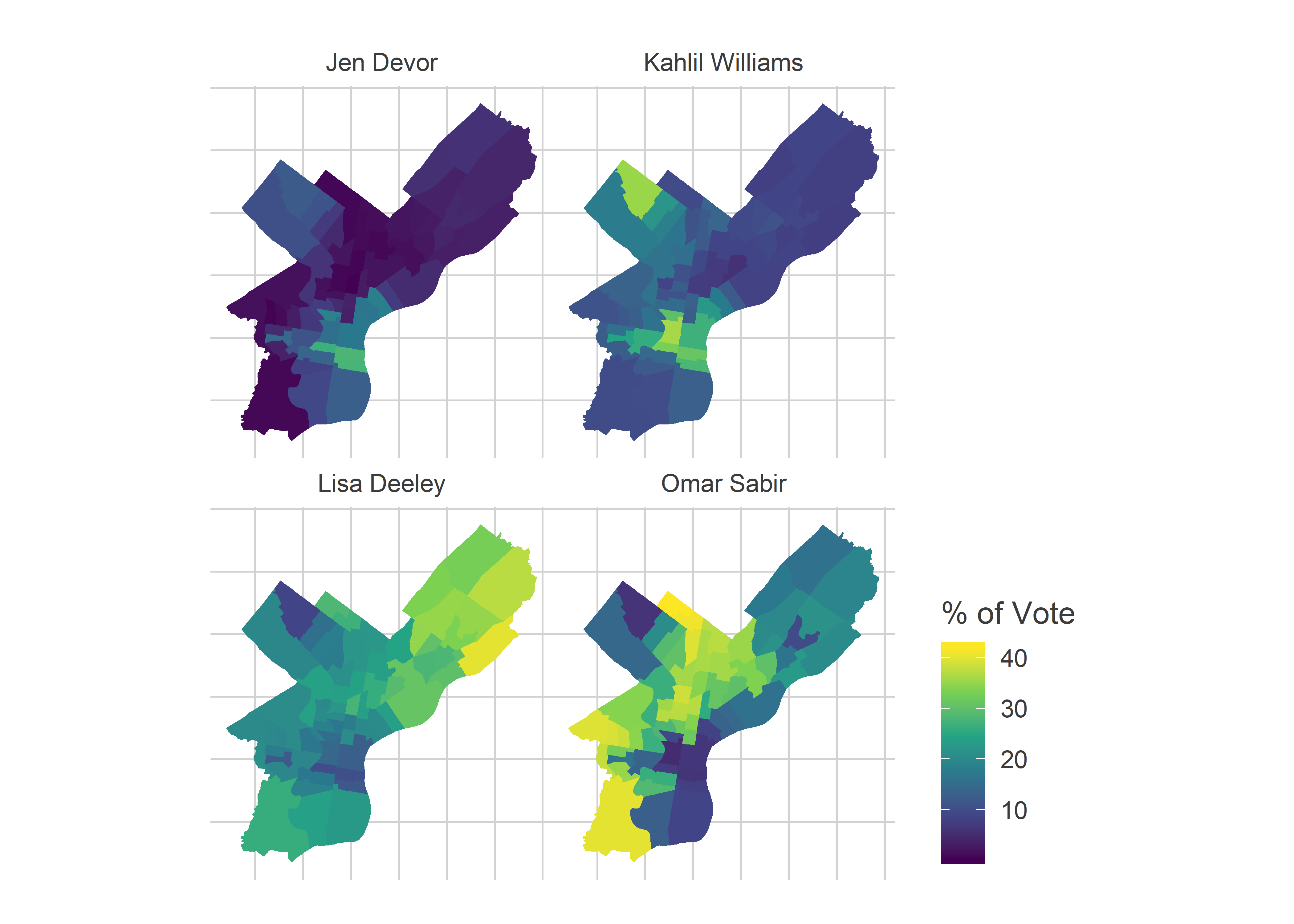
For the Democratic City Council At Large race, the decisive neighborhoods were largely the same. Incumbents Gym, Domb, and Green won across the city, but the two new winners, Thomas and Gilmore Richardson received their highest percents in the Black Voter divisions, while the closest runners up received theirs from the Wealthy Progressives.
(Note: I’ll use the city voting blocs that I’ve discussed before.)
Consider the last in, Gilmore Richardson, versus the first out, Justin DiBerardinis. Gilmore Richardson had more even support across the city than Sabir did, while DiBerardinis attempted to consolidate the Center City and Chestnut Hill/Mount Airy votes, but fell short.
2019 Council Results
View code
council_maps <- map_candidates(
  c("GILMORE RICHARDSON$", "DIBERARDINIS$"),
  yr=2019,
  max_value=0.2
)
council_maps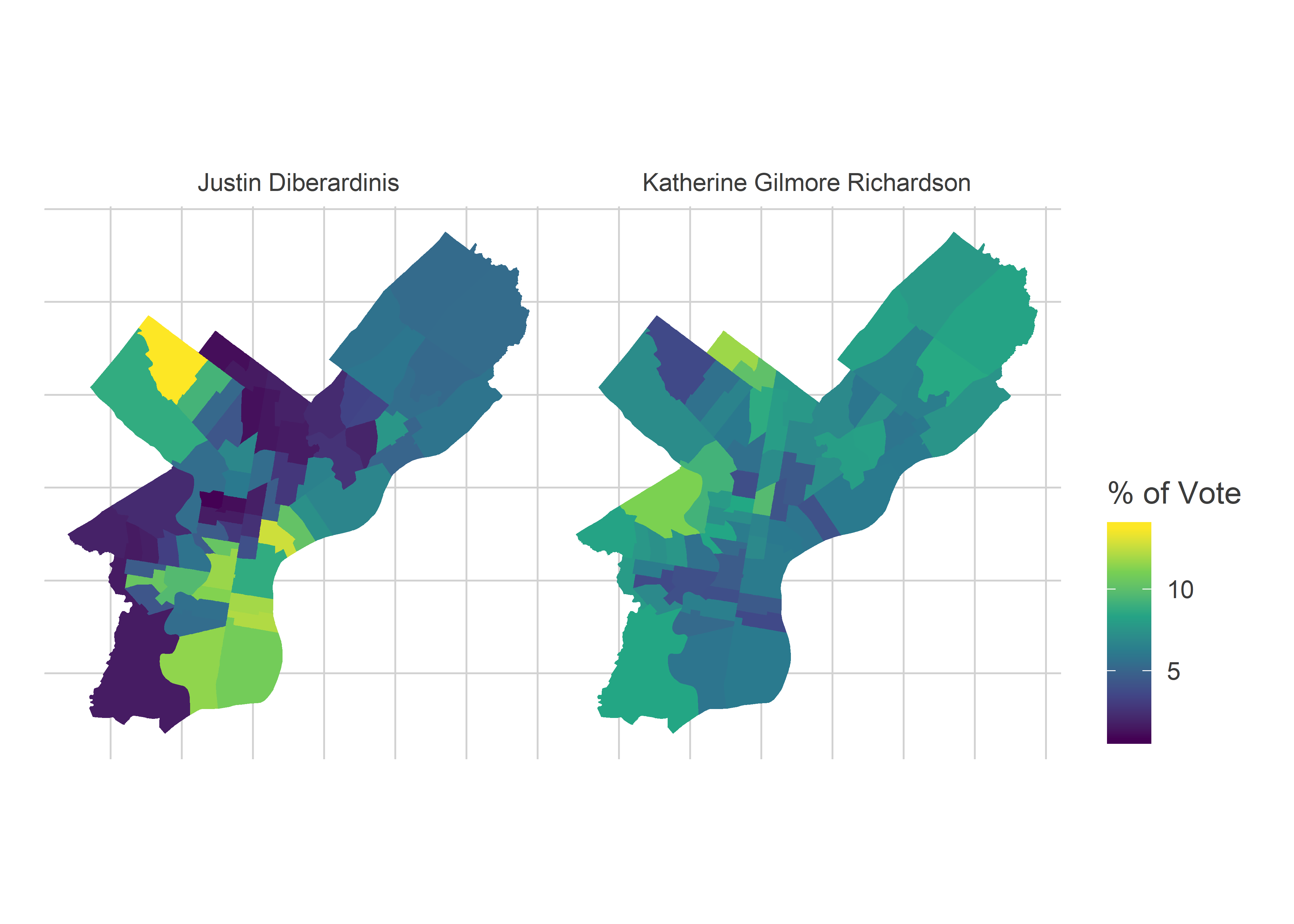
Finally, what did this look like for Common Pleas? Let’s look at four salient candidates: Jennifer Schultz, James Crumlish, Tiffany Palmer, and Kay Yu. The first three won, Yu lost.
2019 Common Pleas Results
View code
commonpleas_maps <- map_candidates(
  c("SCHULTZ$", "ROBERTS$", "PALMER$", "YU$"),
  yr=2019,
  max_value=0.2
)
commonpleas_maps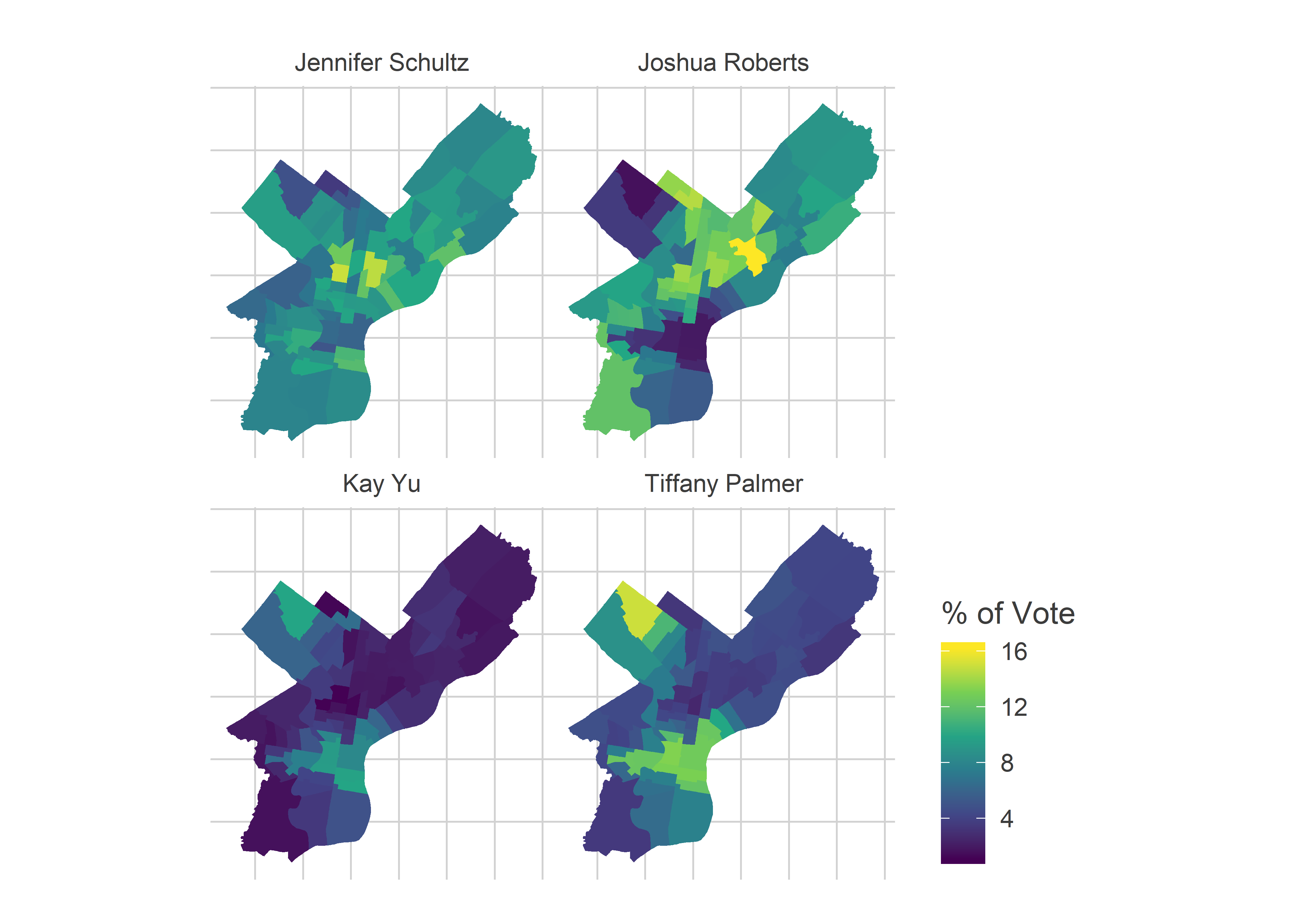
Schultz, with the first ballot position, did well across the city, but especially North Philly. Roberts won places where the DCC nomination matters a lot: the Black Voter and White Moderate divisions. Palmer won a seat with the Wealthy Progressive divisions; Yu’s map looked similar, but she lost.
In some races monopolizing the Wealthy Progressive vote worked, but in other races the votes of the Black Voter divisions dominated. What differentiated them?
Vote power difference by office
My first thought: maybe races have different numbers of votes. Residents could vote for two candidates for Commissioner, five for Council, and six for Common Pleas. In no neighborhoods do voters always vote for the maximum. If voters in different neighborhoods voted for different numbers of candidates, their electoral strength could diverge from just the turnout.
View code
divs_svd <- safe_load("../quick_election_night_maps/divs_svd.Rda") %>%
mutate(warddiv = paste0(substr(warddiv, 1, 2), substr(warddiv,4,5)))
divs_svd$cat <- forcats::fct_recode(
divs_svd$cat,
"Black Voters"="Black non-wealthy",
"Wealthy Progressives"="Wealthy",
"White Moderates"="White non-wealthy"
)
cat_colors <- c(light_blue, light_red, light_orange, light_green)
names(cat_colors) <- levels(divs_svd$cat)
turnout <- safe_load("../voter_db/outputs/turnout_19.rda") %>%
group_by() %>%
filter(`Party Code` == "D")
votes_per_office <- df %>%
filter(year == 2019) %>%
filter(!is.na(office)) %>%
group_by(warddiv, office) %>%
summarise(votes = sum(votes)) %>%
group_by() %>%
left_join(turnout) %>%
left_join(
divs_svd %>% as.data.frame() %>% select(warddiv, cat)
) %>%
group_by(cat, office) %>%
summarise(votes=sum(votes), turnout=sum(turnout)) %>%
group_by() %>%
mutate(votes_per_voter = votes / turnout) %>%
select(cat, votes, turnout, office, votes_per_voter)
# votes_per_office %>% filter(office == "Mayor") %>%
# mutate(pturnout = turnout/sum(turnout))
#
# votes_per_office %>% group_by(office) %>%
# mutate(pvotes = votes/sum(votes))
ggplot(
votes_per_office %>% left_join(office_df),
aes(x=cat, y=votes_per_voter, fill=cat)
) +
geom_bar(stat="identity") +
geom_point(aes(y=nwinners), color=NA) +
geom_text(
aes(label = sprintf("%0.2f", votes_per_voter)),
y=0, vjust=-0.4, color="white"
)+
facet_wrap(~office, scales = "free_y") +
scale_fill_manual(NULL, values=cat_colors) +
theme_sixtysix() %+replace%
theme(axis.text.x = element_blank()) +
ylab("Votes / Voter") +
xlab(NULL) +
ggtitle("Votes per voter in different neighborhood blocs")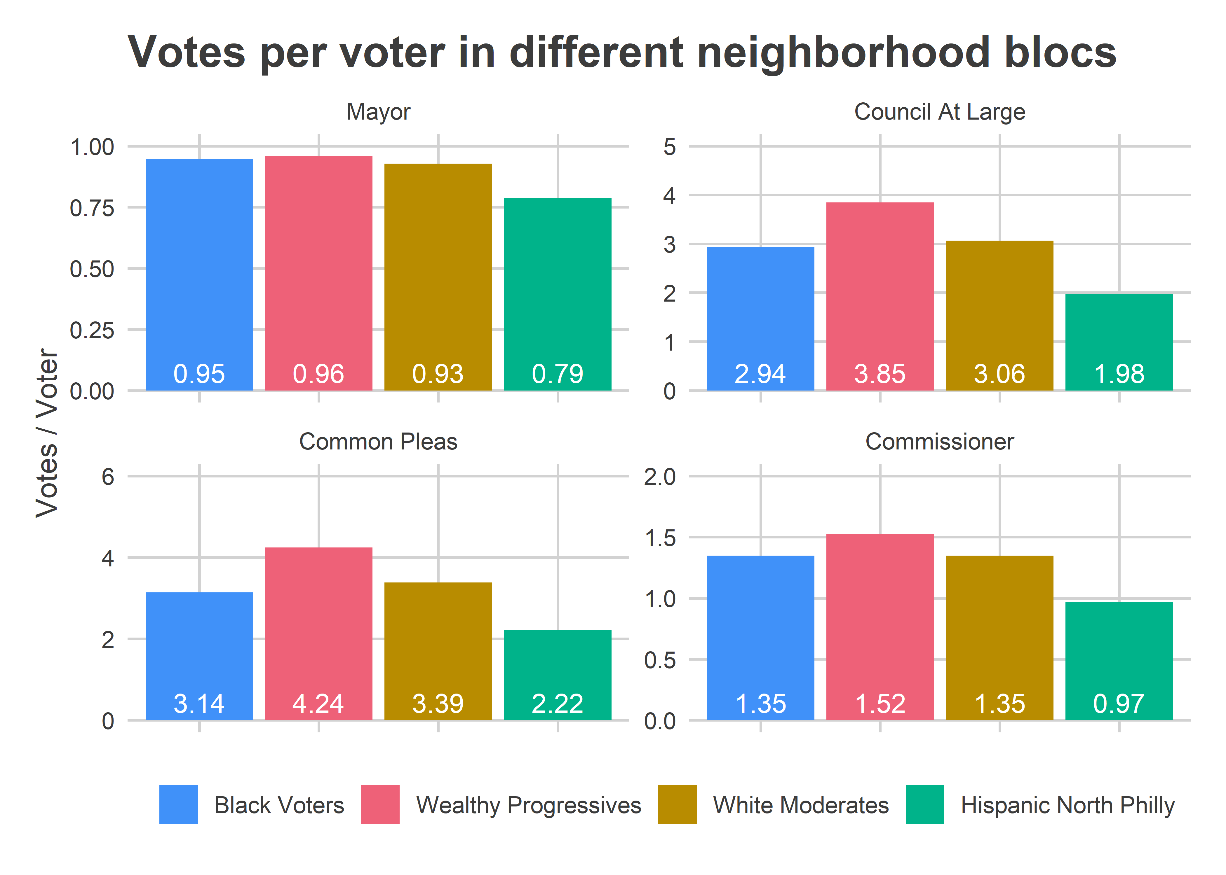 Voting blocs’ numbers are very different by office. The average voter in Black and Wealthy Progressive divisions cast 0.95 and 0.96 votes for Mayor, meaning about 5% of the people who entered the booth left it empty. The rate was basically the same among Black, Wealthy Progressive, and White Moderate divisions.
The rates were not constant for Commissioner. Wealthy Progressive divisions cast 1.52 votes per voter (out of an allowed 2), while Black Voter divisions only cast 1.35.
Wealthy divisions increased that gap even more for Council (voting for 3.9 versus 2.9) and then more for Common Pleas (voting for 4.2 versus 3.1).
Note that I don’t have data for individual voters, so I can’t tell whether this is because some voters skip the race altogether (some vote for 0, others for the full allowance), versus all voters under-voting. We’d need the Commissioner’s Bullet Voting data to adjudicate.
The difference in votes per voter meant that Wealthy Progressive divisions made up 26% of the voters, 26% of the votes for Mayor, 28% of the votes for Commissioner, 31% of the votes for Council at Large, and 32% of the votes for Common Pleas (the Black Voter divisions were 49, 50, 48, 46, and 45, respectively). That’s roughly in order of where their candidates did better: Commissioner worst, Common Pleas best. But the effect isn’t close to strong enough to drive wins except in the narrowest of margins.
One way to visualize that is with scatter plots.
Scatter plots and win lines
I’ve done this before for the Council District Profiles: a twoway scatter mapping the voting blocs of a race. In this case, I’ll plot candidates using their Wealthy Progressive percent on the x-axis, and Black Voter percent on the y-axis. Candidates to the top right do well in both, and win.
View code
cat_df <- df %>%
  filter(year == 2019) %>%
  mutate(candidate_name = format_name(CANDIDATE)) %>%
  filter(!is.na(office)) %>%
  left_join(
    divs_svd %>% as.data.frame() %>% select(warddiv, cat)
  ) %>%
  group_by(office, candidate_name, cat) %>%
  summarise(votes = sum(votes)) %>%
  group_by(office, cat) %>%
  mutate(
    pvote = votes/sum(votes),
    cat_rank = rank(desc(votes), ties.method = "first")
  )

winner_df <- cat_df %>%
  group_by(office, candidate_name) %>%
  summarise(votes = sum(votes)) %>%
  group_by(office) %>%
  mutate(
    pvote = votes/sum(votes),
    office_rank = rank(desc(votes))
  ) %>%
  left_join(office_df) %>%
  mutate(is_winner = office_rank <= nwinners)

win_lines <- winner_df %>%
  filter(office_rank %in% c(nwinners, nwinners+1)) %>%
  group_by(office) %>%
  summarise(win_line = mean(pvote))

slopes <- votes_per_office %>%
  select(cat, office, votes) %>%
  spread(key=cat, value=votes) %>%
  mutate(slope=-`Wealthy Progressives`/`Black Voters`) %>%
  left_join(win_lines) %>%
  mutate(
    intercept = win_line * (`Wealthy Progressives`+`Black Voters`) / `Black Voters`
  )

scatter_df <- cat_df %>%
  filter(candidate_name != "Write In") %>%
  select(-votes) %>%
  rename(rank=cat_rank) %>%
  gather("key", "value", pvote, rank) %>%
  unite("key", cat, key) %>%
  spread(key, value) %>%
  mutate(last_name = format_name(gsub("^.*\\b(\\S+)$", "\\1", candidate_name)))

plot_scatter <- function(use_office){
  max_break <- scatter_df %>%
    filter(office==use_office) %>%
    with(max(c(`Wealthy Progressives_pvote`, `Black Voters_pvote`)))

  breaks <- seq(0,100,by=ifelse(max_break > 0.2, 10, 5))

  ggplot(
    scatter_df %>% filter(office==use_office),
    aes(
      x = 100 * `Wealthy Progressives_pvote`,
      y = 100 * `Black Voters_pvote`
    )
  ) +
    geom_text(
      aes(label = last_name)
    ) +
    geom_abline(
      data=slopes  %>% filter(office==use_office),
      aes(intercept=100*intercept, slope=slope),
      color="grey50",
      linetype="dashed"
    ) +
    # facet_wrap(~office, scales = "free") +
    coord_fixed() +
    scale_x_continuous(
      "Percent of vote among Wealthy Progressive divisions",
      expand=expand_scale(mult=c(0.05, 0.2)),
      breaks=breaks
    ) +
    scale_y_continuous(
      "Percent of vote among Black Voter divisions",
      breaks=breaks
    ) +
    expand_limits(x=0,y=0) +
    theme_sixtysix() +
    ggtitle(sprintf("Voting Bloc results for %s", use_office))
}

plot_scatter("Commissioner")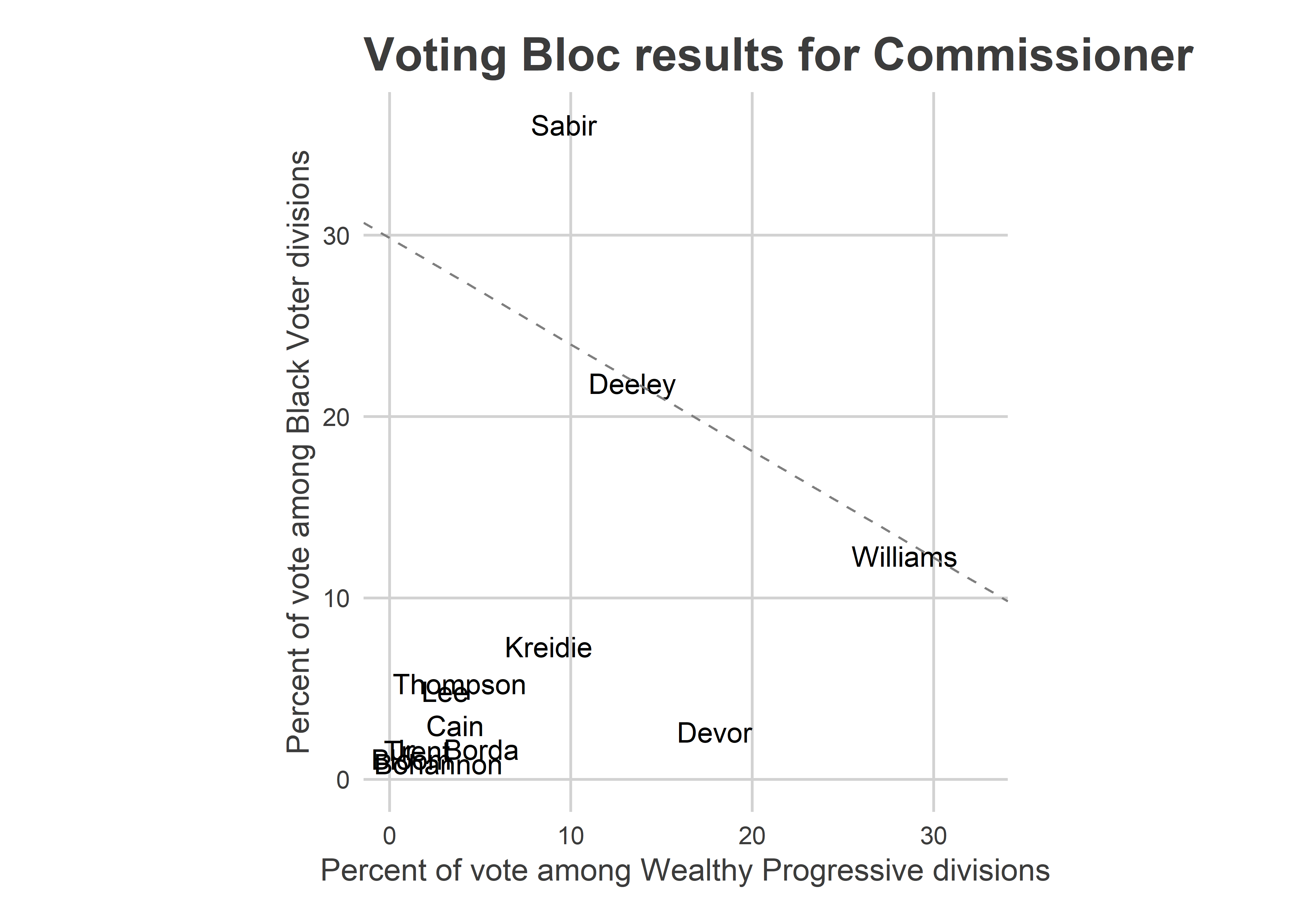
The plot above shows the Commissioner results. The diagonal line is the win line; its slope depends on the relative turnout of the two blocs.
Sabir cleared the line easily, and won. Deeley and Williams ran head-to-head among these blocs (Deeley pulls ahead when you add in the White Moderate divisions).
This race is where the Wealthy Progressive results start to look like vote splitting: Williams and Devor didn’t consolidate the vote of the Wealthy Progressive divisions the way Sabir and Deeley consolidated Black Voter and White Moderate divisions. Had Williams won the 36% among the Wealthy Progressive divisions that Sabir won in Black Voter divisions, that would have been another 6,700 votes. That still wouldn’t have won the race for himc, but would have shrunk the gap behind Deeley by half.
(Note that it’s not clear “vote splitting” happened, since voters could vote for two candidates. So it’s not like the votes for Devor or Kreidie would have otherwise gone to Williams. There probably is at least some substitution effect, though.)
Council has a similar plot, where the runners up clustered just below the line.
View code
plot_scatter("Council At Large")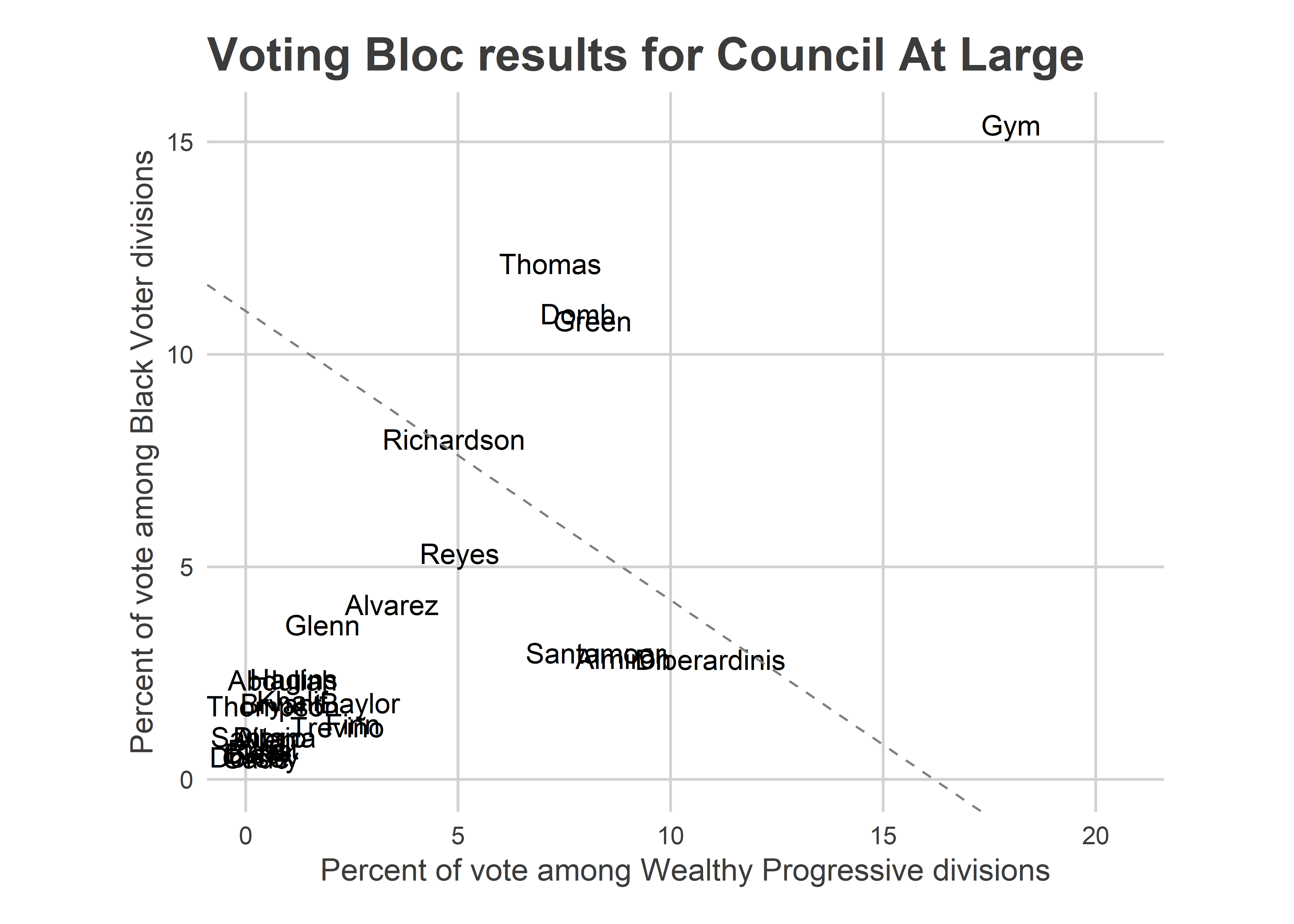 DiBerardinis, Almiron, and Santamoor are the three candidates clustered around 10% in the Wealthy Progressive divisions. Again, we don’t know that they canibalized votes from each other, since voters could choose five candidates. But since voters only pushed the button for 3.85 candidates on average, there was likely substitution among them happening (plus Gym). Of course, Thomas, Domb, and Green also did relatively well in the Wealthy Progressive divisions, which made their overall wins dominant.
For Common Pleas:
View code
plot_scatter("Common Pleas")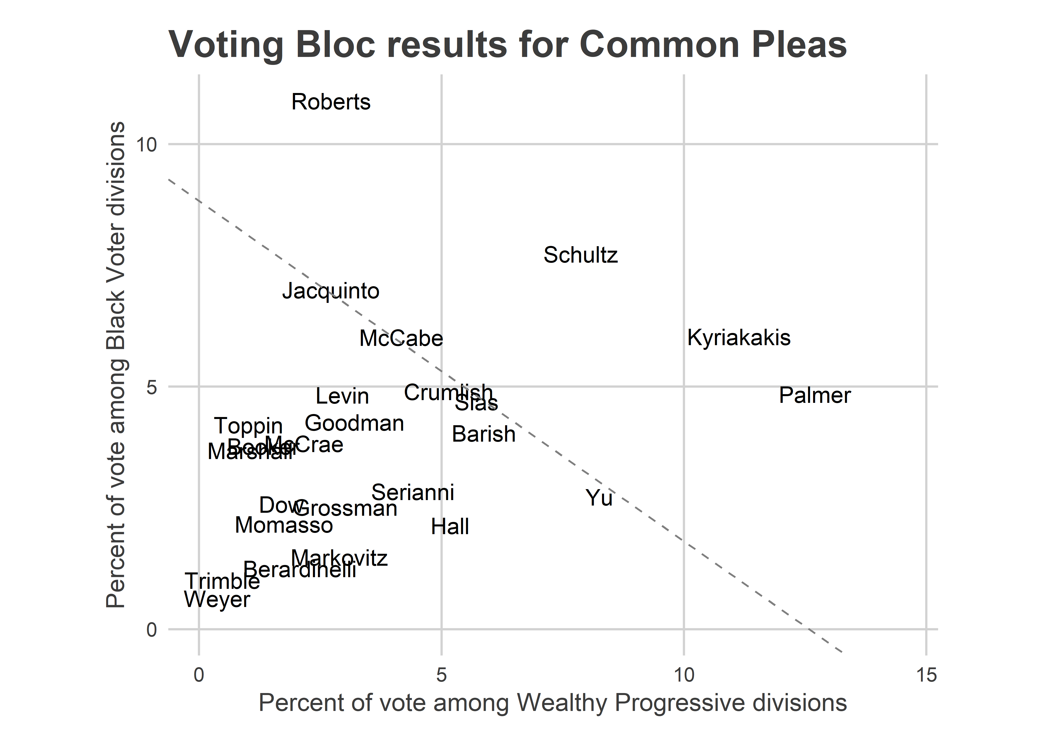
This plot makes it seem that maybe Common Pleas wasn’t different from the other races after all. My original intuition that CP was different was that because the Highly Recommended candidates did so well, and because of Tiffany Palmer’s map, Wealthy Progressives were the determining factor. But this plot shows that they didn’t win solely on the back of Wealthy Progressive neighborhoods. Instead, Palmer finished a strong 7th place among Black Voter divisions, too. The last two judges to win, Crumlish and Jacquinto, were 6th and 3rd in Black Voter divisions, respectively.
Consolidating the vote
One last way to understand vote splitting is a plot of the concentrations of votes in each division. If a voting bloc were able to coordinate their votes so that, for example, their top five Council candidates received 20% of the vote each and everyone else received 0%, that would maximize their power versus the other blocs. If instead they “waste” votes on the sixth and later, then blocs that better consolidate will have more power. Obviously, perfect consolidation won’t happen, but we can look at what percent of the total vote was captured by the winning candidates in each group.
Vote concentration can give a hint at vote splitting. But again, calling it vote splitting assumes that the voters within a bloc have the same preferences, which obviously isn’t true. If one voting bloc has more diversity among voters’ top candidates, that would also hurt this vote consolidation metric.
View code
plot_office <- "Council At Large"
# cat_df %>%
# filter(office == plot_office) %>%
# group_by(cat) %>%
# summarise(
# pvote_one = sum(pvote * (cat_rank == 1)),
# pvote_winners = sum(pvote * (cat_rank > 1 & cat_rank <= 5)),
# pvote_losers = sum(pvote * (cat_rank > 5))
# )
get_office_plot <- function(
plot_office, df=cat_df, title="Vote Concentration for %s", show_appendix_text=TRUE
){
ggplot(
df %>% filter(office == plot_office),
aes(x=cat_rank, y=pvote*100, fill=cat)
) +
geom_bar(stat="identity") +
facet_wrap(~cat) +
scale_fill_manual(NULL, values=cat_colors, guide=FALSE) +
geom_vline(
xintercept=0.5 + office_df$nwinners[office_df$office==plot_office],
linetype="dashed"
) +
theme_sixtysix() %+replace%
theme(axis.text.x = element_blank()) +
xlab(
paste0(
"Candidates sorted by within-cluster rank",
ifelse(show_appendix_text, "\n(See appendix for names and counts.)", "")
)
) +
ylab("Percent of Vote") +
ggtitle(
sprintf(title, plot_office)
)
}
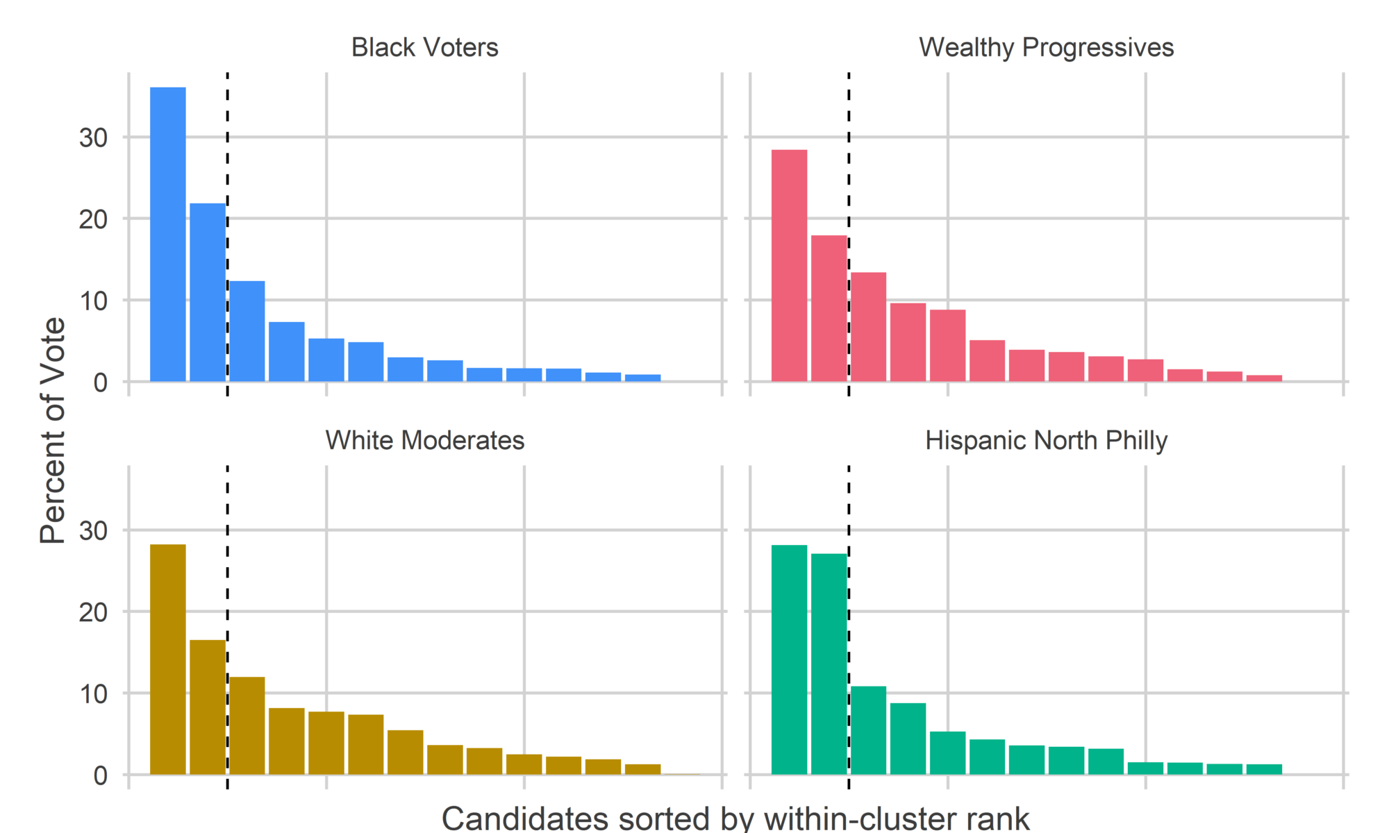
get_office_plot("Council At Large")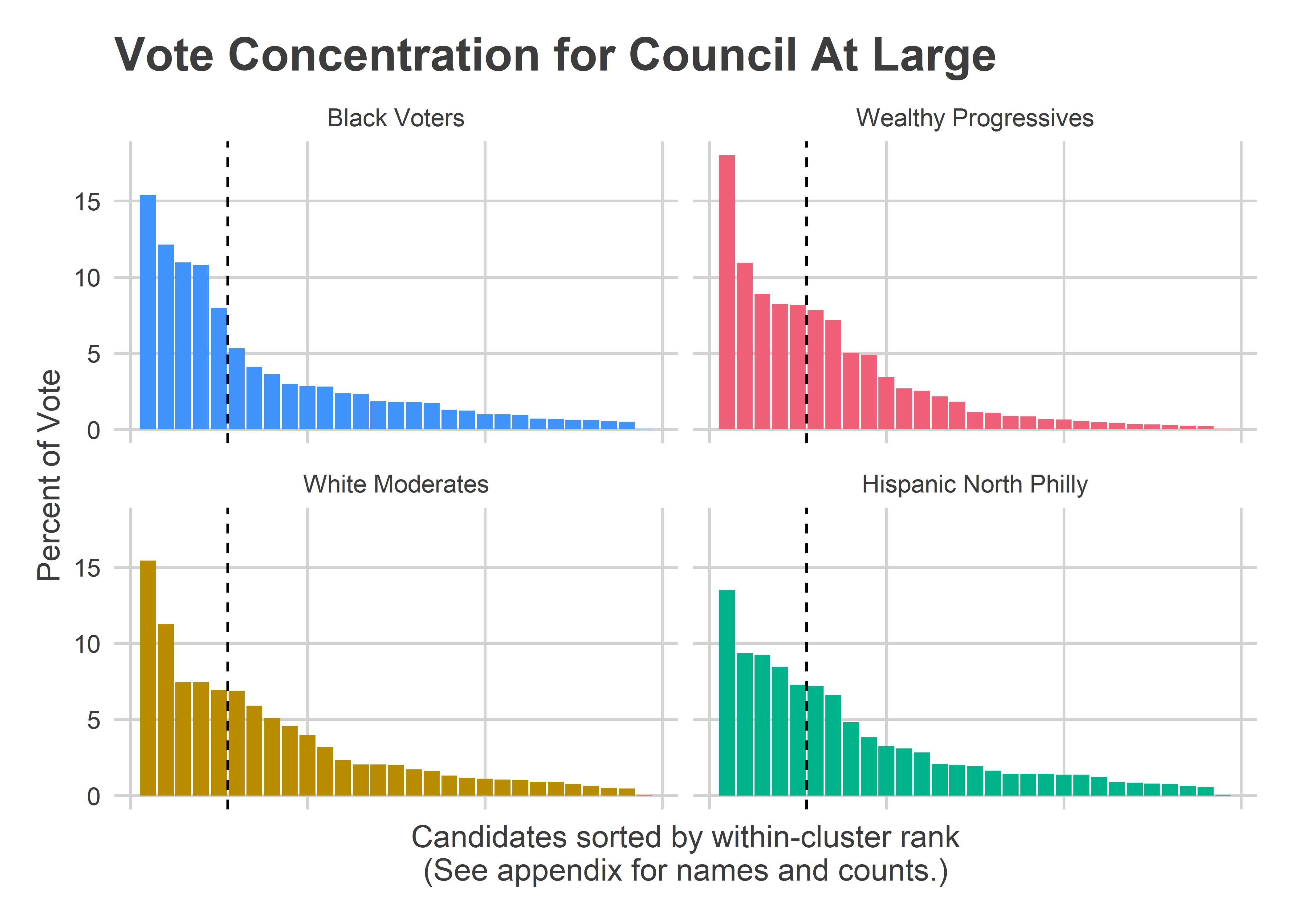
The Black Voter divisions cast 40% of their votes for their 2nd-5th candidates, and 45% of their votes for candidates 6+. The Wealthy Progressive divisions cast 36% of their votes for 2-5, and 46% of their votes for candidates 6+ (Helen Gym was 1st in all of the divisions, and skews the numbers). (For a table with the data behind these plots, see the Appendix.)
Four years ago, those numbers were 40% for the Black Voter 2-5, and 38% for the White Progressive 2-5. So about half the gap, but not enough to swing the election.
Commissioner is the office where there is the best evidence of Wealthy Progressive vote splitting.
View code
# cat_df %>%
# filter(office == "Commissioner") %>%
# group_by(cat) %>%
# summarise(
# pvote_winners = sum(pvote * (cat_rank <= 2)),
# pvote_losers = sum(pvote * (cat_rank > 2))
# )
get_office_plot("Commissioner")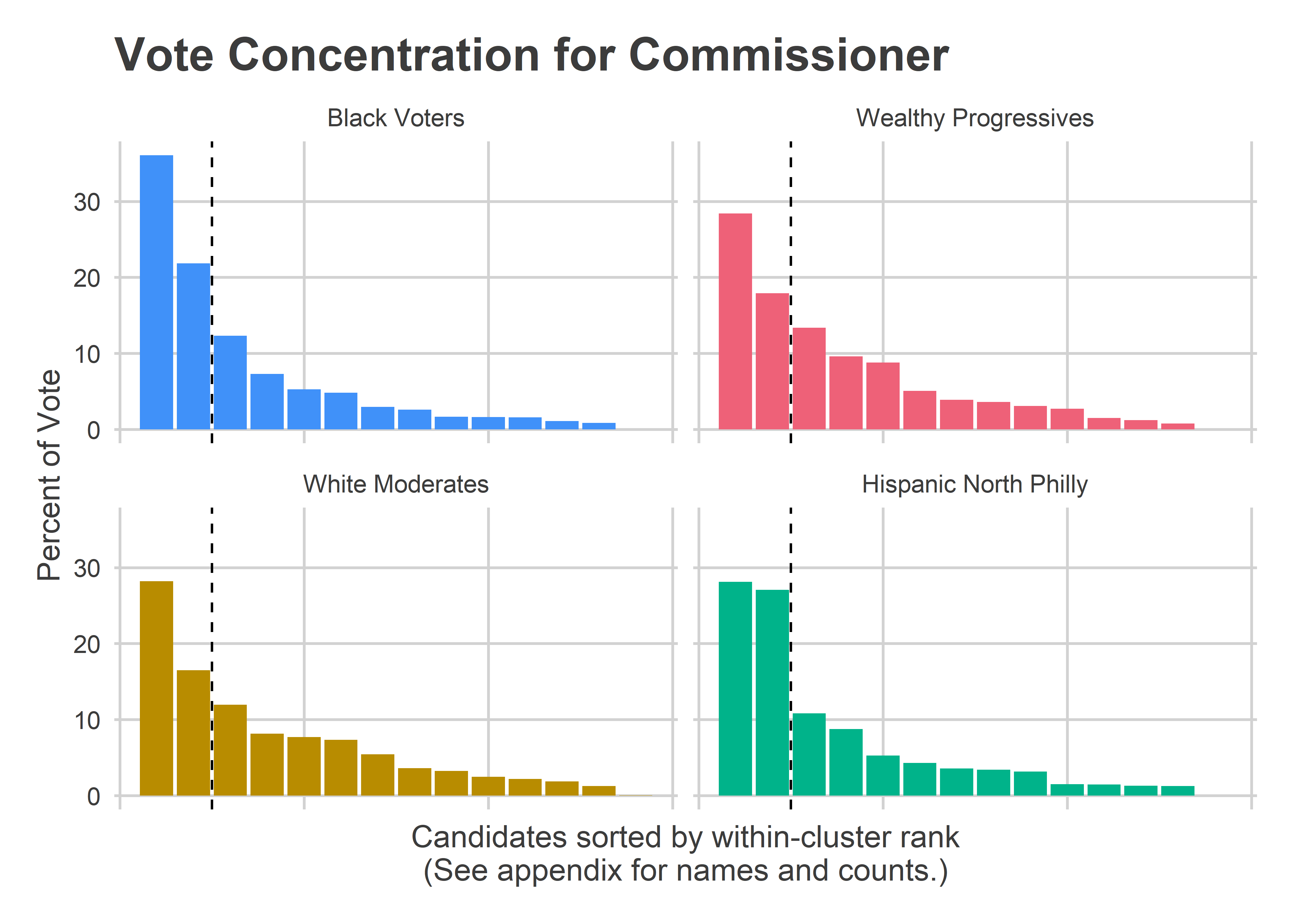 Voters in Black Voter divisions cast 58% of their votes for their two winners, Sabir and Deeley, whereas Wealthy Progressive divisions cast only 46% of their votes for their two, Williams and Devor, and White Moderate divisions only 45%. The fat tail of votes for both the Wealthy Progressives and the White Moderates meant that their favorites received less of a boost.
If Wealthy Progressives had cast their votes for the same ranking of candidates, but using the distribution curve of the Black Voters, then Khalil Williams would have received 6,600 more votes there. This would have been about half of his 12,000 vote city-wide lag.
As I discussed above, it’s not entirely clear that Vote Splitting is the right word for this spreading out of votes. Third and fourth place in the Wealthy Divisions went to Deeley and Sabir, the two winners. So claiming that vote splitting hurt Williams and Devor in these divisions would mean knowing that the votes to the long tail of other candidates would have gone to Williams and Devor, and not Deeley and Sabir.
But Wealthy Progressives did consolidate their vote much more poorly than four years ago. In 2015, Black Voter divisions cast 54% of their vote for their top two commissioners, Wealthy Progressives cast 52%, and White Moderates cast a whopping 58%.
For Common Pleas, the results are exactly the opposite.
View code
# cat_df %>%
# filter(office == "Common Pleas") %>%
# group_by(cat) %>%
# summarise(
# pvote_winners = sum(pvote * (cat_rank <= 6)),
# pvote_losers = sum(pvote * (cat_rank > 6))
# )
get_office_plot("Common Pleas")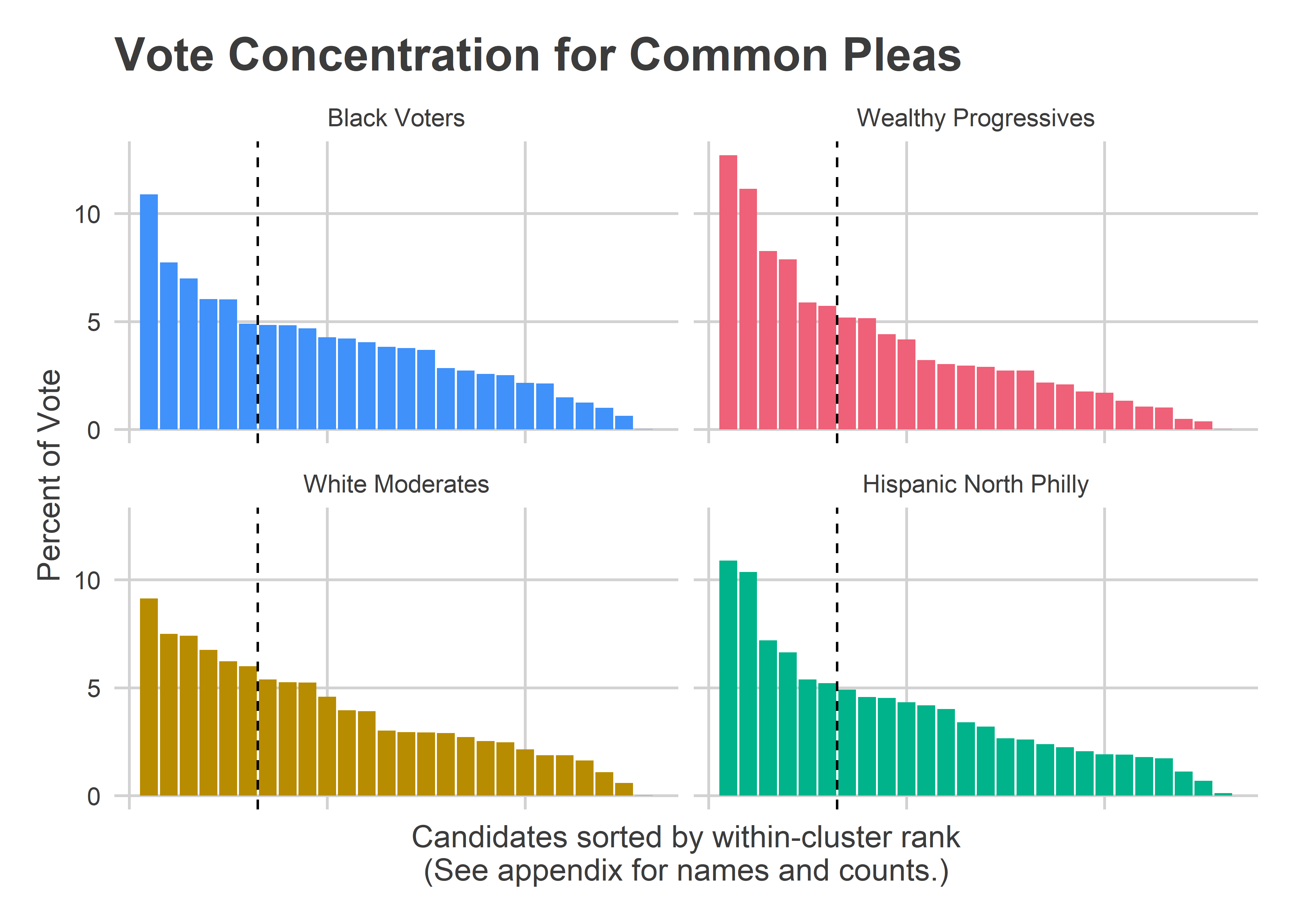 Here, the Black Voters and White Moderates spread out their votes, while the Wealthy Progressive divisions better consolidated their votes to their favored candidates. Those Wealthy Progressives gave 52% of the vote to their cluster winners, and 48% to the rest, while Black Voter and White Moderate divisions only gave 43% to their top six. This concentration of Wealthy Progressive votes is what gave Palmer her dominating win, but it still wasn’t enough for Yu, Barish, and Sias, who were also in the cluster’s top six.
Even with the lower concentration, the sheer vote count power of the Black Voter divisions meant that five of their top six candidates won the city as a whole.
View code
cat_df_15 <- df %>%
  group_by() %>%
  filter(year == 2015) %>%
  mutate(candidate_name = format_name(CANDIDATE)) %>%
  filter(!is.na(office)) %>%
  left_join(
    divs_svd %>% as.data.frame() %>% select(warddiv, cat)
  ) %>%
  group_by(office, candidate_name, cat) %>%
  summarise(votes = sum(votes)) %>%
  group_by(office, cat) %>%
  mutate(
    pvote = votes/sum(votes),
    cat_rank = rank(desc(votes), ties.method = "first")
  )

# cat_df_15 %>%
#   filter(office == "Council At Large") %>%
#   group_by(cat) %>%
#   summarise(
#     pvote_winner = sum(pvote * (cat_rank == 1)),
#     pvote_winners = sum(pvote * (cat_rank <= 5 & cat_rank > 1)),
#     pvote_losers = sum(pvote * (cat_rank > 5))
#   )
#
# cat_df_15 %>%
#   filter(office == "Commissioner") %>%
#   group_by(cat) %>%
#   summarise(
#     pvote_winners = sum(pvote * (cat_rank <= 2)),
#     pvote_losers = sum(pvote * (cat_rank > 2))
#   )
#
# get_office_plot(
#   "Council At Large", cat_df_15, title="Vote Concentration for %s, 2015",
#   show_appendix_text=FALSE
# )
#
# get_office_plot(
#   "Commissioner", cat_df_15, title="Vote Concentration for %s, 2015",
#   show_appendix_text=FALSE
# )
The effect of vote consolidation
The candidates with support in the Black Voter and White Moderate divisions won out in Council and Commissioner. Common Pleas was less clear. Did vote splitting make the difference?
Yes and no.
In Council, the five winners of the Black Voter clusters won the city as a whole, largely thanks to the sheer number of voters there. The vote consolidation wasn’t terribly different from four years ago.
In Common Pleas, the Wealthy Progressives concentrated their vote more than the others, and won for Palmer and Kyriakakis who had unlucky ballot positions. But the winners of Black Voter divisions also won; it turns out the voting blocs just didn’t disagree all that much.
Commissioner saw the largest consolidation effect. Sabir and Deeley won by dominating the Black Voter and White Moderate divisions, respectively. Williams and Devor, the two Wealthy Progressive division winners, finished third and fourth overall, partially because of a lack of Wealthy Progressive consolidation. Had those divisions concentrated their votes similarly to 2015, Williams and Devor each would have received 1,600 more votes. A sizeable chunk, but not enough to change the election.
Appendix: Cluster Result Tables
View code
format_columns <- function(table, cols, ...){
  for(col in cols){
    table <- table %>%
      kableExtra::column_spec(column=col, ...)
  }
  return(table)
}
library(knitr)
library(kableExtra)
get_table_for_office <- function(plot_office){
  overall_df <- cat_df %>%
    group_by() %>%
    filter(office == plot_office) %>%
    group_by(office, candidate_name) %>%
    summarise(votes = sum(votes)) %>%
    group_by() %>%
    mutate(
      cat="Overall",
      pvote = votes/sum(votes),
      cat_rank=rank(desc(votes), ties.method = "first")
    )

  table <- kable(
    cat_df %>%
      group_by() %>%
      filter(office == plot_office) %>%
      bind_rows(overall_df) %>%
      mutate(
        cat=factor(cat, levels=c("Overall", names(cat_colors))),
        votes=paste0(scales::comma(votes), " (", round(100 * pvote),"%)")
      ) %>%
      select(candidate_name, cat, votes, cat_rank) %>%
      rename(
        "Rank in Cluster" = cat_rank,
        "Candidate" = candidate_name
      ) %>%
      gather("key", "value", Candidate, votes) %>%
      mutate(key = format_name(key), blank="     ") %>%
      unite(key, cat, key, sep=": ") %>%
      spread(key, value) %>%
      select(
        "Rank in Cluster",
        blank,
        starts_with("Overall"),
        starts_with("Black"),
        starts_with("Wealthy"),
        starts_with("White"),
        starts_with("Hispanic")
      )
    ,
    caption=sprintf("Cluster Results for %s", plot_office),
    align='l',
    col.names=c("Rank","", rep(c("Candidate", "Votes"), times=5)),
    padding = "4in"
  ) %>%
    column_spec(2, width = "1em") %>%
    add_header_above(
      c(" " = 2, "Overall" = 2, "Black Voters" = 2, "Wealthy Progressives" = 2,
        "White Moderates" = 2, "Hispanic North Philly" = 2)
    ) %>%
    kable_styling() %>%
    scroll_box(width="100%")

  return(table)
}

get_table_for_office("Commissioner")| Rank | Candidate | Votes | Candidate | Votes | Candidate | Votes | Candidate | Votes | Candidate | Votes | |
|---|---|---|---|---|---|---|---|---|---|---|---|
| 1 | Omar Sabir | 71,303 (24%) | Omar Sabir | 50,859 (36%) | Kahlil Williams | 23,546 (28%) | Lisa Deeley | 16,955 (28%) | Omar Sabir | 2,559 (28%) | |
| 2 | Lisa Deeley | 61,278 (21%) | Lisa Deeley | 30,766 (22%) | Jen Devor | 14,853 (18%) | Omar Sabir | 9,909 (16%) | Lisa Deeley | 2,465 (27%) | |
| 3 | Kahlil Williams | 48,884 (17%) | Kahlil Williams | 17,346 (12%) | Lisa Deeley | 11,092 (13%) | Kahlil Williams | 7,193 (12%) | Marwan Kreidie | 984 (11%) | |
| 4 | Jen Devor | 23,752 (8%) | Marwan Kreidie | 10,295 (7%) | Omar Sabir | 7,976 (10%) | Jen Devor | 4,905 (8%) | Kahlil Williams | 799 (9%) | |
| 5 | Marwan Kreidie | 23,190 (8%) | Annette Thompson | 7,422 (5%) | Marwan Kreidie | 7,278 (9%) | Marwan Kreidie | 4,633 (8%) | Annette Thompson | 480 (5%) | |
| 6 | Annette Thompson | 14,389 (5%) | Dennis Lee | 6,828 (5%) | Luigi Borda | 4,210 (5%) | Luigi Borda | 4,422 (7%) | Luigi Borda | 390 (4%) | |
| 7 | Dennis Lee | 11,649 (4%) | Carla Cain | 4,161 (3%) | Annette Thompson | 3,217 (4%) | Annette Thompson | 3,270 (5%) | Jen Devor | 325 (4%) | |
| 8 | Luigi Borda | 11,352 (4%) | Jen Devor | 3,669 (3%) | Carla Cain | 3,004 (4%) | Carla Cain | 2,160 (4%) | Dennis Lee | 309 (3%) | |
| 9 | Carla Cain | 9,613 (3%) | Luigi Borda | 2,330 (2%) | Dennis Lee | 2,558 (3%) | Dennis Lee | 1,954 (3%) | Carla Cain | 288 (3%) | |
| 10 | Moira Bohannon | 5,054 (2%) | Lewis Harris Jr | 2,292 (2%) | Moira Bohannon | 2,247 (3%) | Moira Bohannon | 1,485 (2%) | Robin Trent | 136 (1%) | |
| 11 | Robin Trent | 4,949 (2%) | Robin Trent | 2,239 (2%) | Robin Trent | 1,259 (2%) | Robin Trent | 1,315 (2%) | Moira Bohannon | 133 (1%) | |
| 12 | Warren Bloom | 3,808 (1%) | Warren Bloom | 1,563 (1%) | Warren Bloom | 1,001 (1%) | Warren Bloom | 1,124 (2%) | Warren Bloom | 120 (1%) | |
| 13 | Lewis Harris Jr | 3,793 (1%) | Moira Bohannon | 1,189 (1%) | Lewis Harris Jr | 627 (1%) | Lewis Harris Jr | 758 (1%) | Lewis Harris Jr | 116 (1%) | |
| 14 | Write In | 34 (0%) | Write In | 10 (0%) | Write In | 4 (0%) | Write In | 19 (0%) | Write In | 1 (0%) |
View code
get_table_for_office("Council At Large")| Rank | Candidate | Votes | Candidate | Votes | Candidate | Votes | Candidate | Votes | Candidate | Votes | |
|---|---|---|---|---|---|---|---|---|---|---|---|
| 1 | Helen Gym | 108,604 (16%) | Helen Gym | 47,309 (15%) | Helen Gym | 37,687 (18%) | Helen Gym | 21,087 (15%) | Helen Gym | 2,521 (14%) | |
| 2 | Allan Domb | 67,193 (10%) | Isaiah Thomas | 37,294 (12%) | Justin Diberardinis | 22,895 (11%) | Allan Domb | 15,403 (11%) | Allan Domb | 1,747 (9%) | |
| 3 | Isaiah Thomas | 64,045 (10%) | Allan Domb | 33,664 (11%) | Erika Almirón | 18,618 (9%) | Justin Diberardinis | 10,190 (7%) | Adrián Rivera-Reyes | 1,720 (9%) | |
| 4 | Derek S Green | 61,070 (9%) | Derek S Green | 33,145 (11%) | Eryn Santamoor | 17,209 (8%) | Isaiah Thomas | 10,173 (7%) | Isaiah Thomas | 1,576 (8%) | |
| 5 | Katherine Gilmore Richardson | 45,470 (7%) | Katherine Gilmore Richardson | 24,581 (8%) | Derek S Green | 17,085 (8%) | Derek S Green | 9,496 (7%) | Deja Lynn Alvarez | 1,359 (7%) | |
| 6 | Justin Diberardinis | 42,643 (6%) | Adrián Rivera-Reyes | 16,323 (5%) | Allan Domb | 16,379 (8%) | Katherine Gilmore Richardson | 9,396 (7%) | Derek S Green | 1,344 (7%) | |
| 7 | Adrián Rivera-Reyes | 35,565 (5%) | Deja Lynn Alvarez | 12,638 (4%) | Isaiah Thomas | 15,002 (7%) | Eryn Santamoor | 8,084 (6%) | Katherine Gilmore Richardson | 1,232 (7%) | |
| 8 | Eryn Santamoor | 35,026 (5%) | Sandra Dungee Glenn | 11,153 (4%) | Adrián Rivera-Reyes | 10,545 (5%) | Adrián Rivera-Reyes | 6,977 (5%) | Justin Diberardinis | 899 (5%) | |
| 9 | Erika Almirón | 34,329 (5%) | Eryn Santamoor | 9,129 (3%) | Katherine Gilmore Richardson | 10,261 (5%) | Erika Almirón | 6,254 (5%) | Erika Almirón | 715 (4%) | |
| 10 | Deja Lynn Alvarez | 26,617 (4%) | Erika Almirón | 8,742 (3%) | Deja Lynn Alvarez | 7,190 (3%) | Deja Lynn Alvarez | 5,430 (4%) | Eryn Santamoor | 604 (3%) | |
| 11 | Sandra Dungee Glenn | 18,105 (3%) | Justin Diberardinis | 8,659 (3%) | Ethelind Baylor | 5,646 (3%) | Beth Finn | 4,333 (3%) | Ogbonna Paul Hagins | 576 (3%) | |
| 12 | Ethelind Baylor | 14,259 (2%) | Ogbonna Paul Hagins | 7,260 (2%) | Beth Finn | 5,281 (3%) | Joseph A Diorio | 3,186 (2%) | Fernando Treviño | 530 (3%) | |
| 13 | Beth Finn | 14,015 (2%) | Fareed Abdullah | 7,170 (2%) | Fernando Treviño | 4,519 (2%) | Ethelind Baylor | 2,808 (2%) | Beth Finn | 389 (2%) | |
| 14 | Ogbonna Paul Hagins | 12,570 (2%) | Asa Khalif | 5,682 (2%) | Sandra Dungee Glenn | 3,795 (2%) | Fernando Treviño | 2,799 (2%) | Sandra Dungee Glenn | 379 (2%) | |
| 15 | Fernando Treviño | 11,646 (2%) | Ethelind Baylor | 5,535 (2%) | Ogbonna Paul Hagins | 2,369 (1%) | Sandra Dungee Glenn | 2,778 (2%) | Joseph A Diorio | 358 (2%) | |
| 16 | Fareed Abdullah | 10,676 (2%) | Latrice Y Bryant | 5,473 (2%) | Asa Khalif | 2,303 (1%) | Ogbonna Paul Hagins | 2,365 (2%) | Billy Thompson | 306 (2%) | |
| 17 | Asa Khalif | 9,779 (1%) | Billy Thompson | 5,300 (2%) | Fareed Abdullah | 1,821 (1%) | Billy Thompson | 2,205 (2%) | Ethelind Baylor | 270 (1%) | |
| 18 | Billy Thompson | 9,166 (1%) | Beth Finn | 4,012 (1%) | Latrice Y Bryant | 1,773 (1%) | Vinny Black | 1,801 (1%) | Edwin Santana | 269 (1%) | |
| 19 | Latrice Y Bryant | 8,966 (1%) | Fernando Treviño | 3,798 (1%) | Hena Veit | 1,413 (1%) | Hena Veit | 1,620 (1%) | Latrice Y Bryant | 269 (1%) | |
| 20 | Joseph A Diorio | 7,803 (1%) | Edwin Santana | 3,061 (1%) | Billy Thompson | 1,355 (1%) | Asa Khalif | 1,538 (1%) | Fareed Abdullah | 258 (1%) | |
| 21 | Hena Veit | 5,474 (1%) | Joseph A Diorio | 3,054 (1%) | Joseph A Diorio | 1,205 (1%) | Latrice Y Bryant | 1,451 (1%) | Asa Khalif | 256 (1%) | |
| 22 | Edwin Santana | 5,272 (1%) | Wayne Allen | 2,926 (1%) | Wayne Allen | 958 (0%) | Fareed Abdullah | 1,427 (1%) | Hena Veit | 232 (1%) | |
| 23 | Wayne Allen | 4,941 (1%) | Hena Veit | 2,209 (1%) | Edwin Santana | 883 (0%) | Bobbie Curry | 1,255 (1%) | Vinny Black | 168 (1%) | |
| 24 | Vinny Black | 4,516 (1%) | Mark Ross | 2,137 (1%) | Mark Ross | 722 (0%) | Mark Ross | 1,253 (1%) | Wayne Allen | 158 (1%) | |
| 25 | Mark Ross | 4,255 (1%) | Bobbie Curry | 1,923 (1%) | Vinny Black | 685 (0%) | Edwin Santana | 1,059 (1%) | Bobbie Curry | 146 (1%) | |
| 26 | Bobbie Curry | 3,920 (1%) | Vinny Black | 1,862 (1%) | Bobbie Curry | 596 (0%) | Wayne Allen | 899 (1%) | Mark Ross | 143 (1%) | |
| 27 | Devon Cade | 2,854 (0%) | Wayne Edmund Dorsey | 1,606 (1%) | Devon Cade | 522 (0%) | Devon Cade | 683 (0%) | Devon Cade | 116 (1%) | |
| 28 | Wayne Edmund Dorsey | 2,780 (0%) | Devon Cade | 1,533 (0%) | Wayne Edmund Dorsey | 428 (0%) | Wayne Edmund Dorsey | 643 (0%) | Wayne Edmund Dorsey | 103 (1%) | |
| 29 | Write In | 316 (0%) | Write In | 127 (0%) | Write In | 101 (0%) | Write In | 77 (0%) | Write In | 11 (0%) |
View code
get_table_for_office("Common Pleas")| Rank | Candidate | Votes | Candidate | Votes | Candidate | Votes | Candidate | Votes | Candidate | Votes | |
|---|---|---|---|---|---|---|---|---|---|---|---|
| 1 | Jennifer Schultz | 59,547 (8%) | Joshua Roberts | 35,820 (11%) | Tiffany Palmer | 29,310 (13%) | Jennifer Schultz | 13,789 (9%) | Joshua Roberts | 2,281 (11%) | |
| 2 | Anthony Kyriakakis | 58,128 (8%) | Jennifer Schultz | 25,424 (8%) | Anthony Kyriakakis | 25,711 (11%) | Joshua Roberts | 11,317 (7%) | Jennifer Schultz | 2,171 (10%) | |
| 3 | Joshua Roberts | 55,702 (8%) | Carmella Jacquinto | 23,005 (7%) | Kay Yu | 19,046 (8%) | Anthony Kyriakakis | 11,187 (7%) | Carmella Jacquinto | 1,506 (7%) | |
| 4 | Tiffany Palmer | 55,586 (8%) | Anthony Kyriakakis | 19,840 (6%) | Jennifer Schultz | 18,163 (8%) | James C Crumlish | 10,203 (7%) | Anthony Kyriakakis | 1,390 (7%) | |
| 5 | James C Crumlish | 39,217 (5%) | Cateria R McCabe | 19,788 (6%) | Wendi Barish | 13,562 (6%) | Tiffany Palmer | 9,392 (6%) | Craig Levin | 1,127 (5%) | |
| 6 | Carmella Jacquinto | 38,920 (5%) | James C Crumlish | 16,107 (5%) | Henry McGregor Sias | 13,202 (6%) | Wendi Barish | 9,062 (6%) | Wendi Barish | 1,092 (5%) | |
| 7 | Wendi Barish | 36,998 (5%) | Tiffany Palmer | 15,927 (5%) | Chris Hall | 11,956 (5%) | Carmella Jacquinto | 8,128 (5%) | James C Crumlish | 1,030 (5%) | |
| 8 | Cateria R McCabe | 36,214 (5%) | Craig Levin | 15,872 (5%) | James C Crumlish | 11,877 (5%) | Beth Grossman | 7,932 (5%) | Tiffany Palmer | 957 (5%) | |
| 9 | Kay Yu | 34,475 (5%) | Henry McGregor Sias | 15,413 (5%) | Nicola Serianni | 10,173 (4%) | Nicola Serianni | 7,923 (5%) | Jon Marshall | 948 (5%) | |
| 10 | Henry McGregor Sias | 33,560 (5%) | Leon Goodman | 14,027 (4%) | Cateria R McCabe | 9,629 (4%) | Craig Levin | 6,916 (5%) | Nicola Serianni | 907 (4%) | |
| 11 | Craig Levin | 30,746 (4%) | Sherman Toppin | 13,854 (4%) | Leon Goodman | 7,394 (3%) | Kay Yu | 5,979 (4%) | Cateria R McCabe | 877 (4%) | |
| 12 | Nicola Serianni | 28,328 (4%) | Wendi Barish | 13,282 (4%) | Beth Grossman | 6,965 (3%) | Cateria R McCabe | 5,920 (4%) | Henry McGregor Sias | 841 (4%) | |
| 13 | Leon Goodman | 26,352 (4%) | Kendra McCrae | 12,585 (4%) | Craig Levin | 6,831 (3%) | Chris Hall | 4,552 (3%) | Beth Grossman | 711 (3%) | |
| 14 | Chris Hall | 23,891 (3%) | Terri M Booker | 12,388 (4%) | Vicki Markovitz | 6,677 (3%) | Vicki Markovitz | 4,445 (3%) | Sherman Toppin | 671 (3%) | |
| 15 | Beth Grossman | 23,876 (3%) | Jon Marshall | 12,105 (4%) | Joshua Roberts | 6,284 (3%) | James F Berardinelli | 4,412 (3%) | Leon Goodman | 556 (3%) | |
| 16 | Kendra McCrae | 21,853 (3%) | Nicola Serianni | 9,325 (3%) | Carmella Jacquinto | 6,281 (3%) | Leon Goodman | 4,375 (3%) | Kendra McCrae | 545 (3%) | |
| 17 | Sherman Toppin | 19,331 (3%) | Kay Yu | 8,950 (3%) | Kendra McCrae | 4,999 (2%) | Henry McGregor Sias | 4,104 (3%) | Kay Yu | 500 (2%) | |
| 18 | Jon Marshall | 19,322 (3%) | Laurie Dow | 8,464 (3%) | James F Berardinelli | 4,792 (2%) | Jon Marshall | 3,823 (3%) | Terri M Booker | 470 (2%) | |
| 19 | Terri M Booker | 18,750 (3%) | Beth Grossman | 8,268 (3%) | Janine D Momasso | 4,052 (2%) | Kendra McCrae | 3,724 (2%) | Vicki Markovitz | 431 (2%) | |
| 20 | Vicki Markovitz | 16,433 (2%) | Janine D Momasso | 7,111 (2%) | Laurie Dow | 3,924 (2%) | Laurie Dow | 3,233 (2%) | Janine D Momasso | 402 (2%) | |
| 21 | Laurie Dow | 16,020 (2%) | Chris Hall | 7,009 (2%) | Terri M Booker | 3,061 (1%) | Terri M Booker | 2,831 (2%) | Laurie Dow | 399 (2%) | |
| 22 | Janine D Momasso | 14,384 (2%) | Vicki Markovitz | 4,880 (1%) | Jon Marshall | 2,446 (1%) | Janine D Momasso | 2,819 (2%) | Chris Hall | 374 (2%) | |
| 23 | James F Berardinelli | 13,663 (2%) | James F Berardinelli | 4,098 (1%) | Sherman Toppin | 2,355 (1%) | Sherman Toppin | 2,451 (2%) | James F Berardinelli | 361 (2%) | |
| 24 | Robert Trimble | 6,305 (1%) | Robert Trimble | 3,300 (1%) | Robert Trimble | 1,123 (0%) | Robert Trimble | 1,649 (1%) | Robert Trimble | 233 (1%) | |
| 25 | Gregory Weyer | 3,962 (1%) | Gregory Weyer | 2,069 (1%) | Gregory Weyer | 861 (0%) | Gregory Weyer | 889 (1%) | Gregory Weyer | 143 (1%) | |
| 26 | Write In | 108 (0%) | Write In | 33 (0%) | Write In | 23 (0%) | Write In | 27 (0%) | Write In | 25 (0%) |