On May 21st, Philadelphia won’t just be voting for Mayor, City Council, and a few “row offices”. Besides those, we will also choose nine judges: two for the Superior Court, one for Municipal Court, and six for the Court of Common Pleas. (Really, this is just the primary. But the Common Pleas and Municipal nominees will almost certainly win in November).
I’ve spent time here before looking at the Court of Common Pleas. The court is responsible for the city’s major civil and criminal trials. Its judges are elected to ten-year terms. And we elect them by drawing out of a coffee can.
The result is that Philadelphia often elects judges who are unfit for the office. In 2015, Scott Diclaudio won; months later he would be censured for misconduct and negligence, and then get caught having given illegal donations in the DA Seth Williams probe. He was in the first position on the ballot. Lyris Younge was at the bottom of the first column that year and won. She has since been removed from Family Court for violating family rights and made headlines by evicting a full building of residents with less than a week’s notice.
I’ve looked before at the effect of ballot position on the Court’s elections: being in the first column nearly triples your votes. Today, I’ll use that model to simulate who will win in the upcoming race.
It’s easy to predict the Common Pleas Election
Predicting elections is hard, especially without surveys. When I tried it for November’s state house election, I could only make imprecise predictions, and even then had mixed results. Why would this time be any different?
The key is that voters know nothing about the race. In May, voters are selecting six Common Pleas judges from among twenty-five candidates. The median voter will know the name of exactly zero of them before they enter the booth.
This lack of knowledge means that structural components end up mattering a lot. What column your name is listed in, whether you’re endorsed in the Inquirer, or how many polling places your name is handed out on a piece of paper outside of, all dictate who will win. We can observe or guess each of those, and come up with pretty accurate predictions.
When I did this exercise two years ago, I got the number of winners from the first column, and the number endorsed by the DCC, exactly right (yes, it’s that easy).
Electing qualified judges
These races matter. Philadelphia regularly elects judges who should not be judges, granting them the authority over a courtroom that decides the city’s most important cases.
As a measure of judicial quality, I use the recommendations from the Judicial Commission of the Philadelphia Bar Association. The commission evaluates candidates by an interview, a questionnaire, and interviews with people who work with them. It then rates candidates as Recommended or Not Recommended. Usually, it recommends about 2/3 of the candidates–many more than can win–and is useful as a lower-bar measure of candidate quality. My understanding is that when a candidate isn’t recommended, there’s a significant reason, though the Commission’s exact findings are kept confidential.
The ratings are so useful that in 2015 the Philadelphia Inquirer stopped endorsing judicial candidates on its own, and began printing the Commission’s recommendations (this also makes the ratings much more important for candidates).
Recently, the Commission introduced a Highly Recommended category. Unfortunately, it’s too early to know how effective it’s been. In 2015 there were three Highly Recommended candidates, and all three won. But they didn’t do statistically significantly better than the plain old Recommended Candidates in terms of votes (albeit with just three observations). In 2017, there were no Highly Recommended candidates.
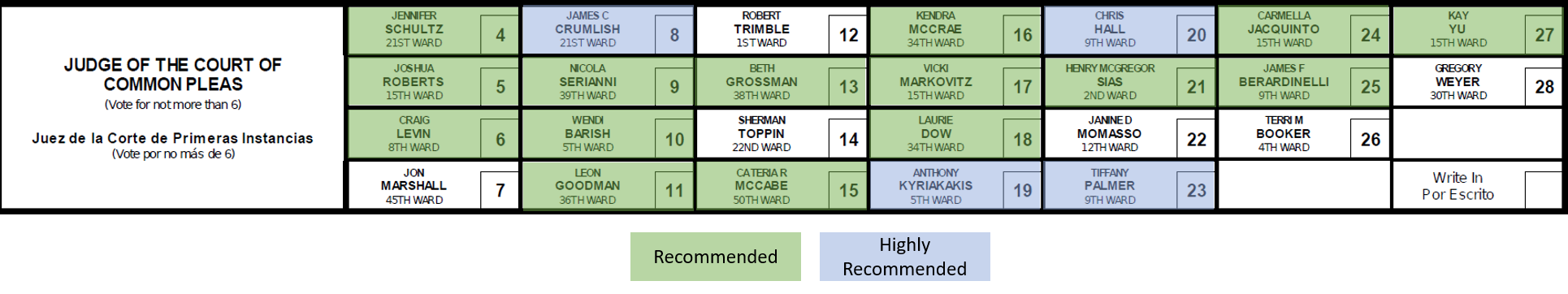
This time around, there are four Highly Recommended candidates: James Crulish, Anthony Kyriakakis, Chris Hall, and Tiffany Palmer (a fifth, Michelle Hangley, dropped out because of her unlucky ballot position). None of those four are in the first column, so this year could prove a useful measure of the Bar’s impact.
One note: candidates that do not submit questionnaires are not rated Recommended. Rather than reward the perverse incentive for candidates to not submit, I will consider candidates who have not yet submitted paperwork as Not Recommended.
Where will ballot position matter most?
When I analysed the determinants of Common Pleas voting, being in the first column nearly tripled a candidate’s votes. Endorsements from the Democratic City Committee (DCC) and the Inquirer doubled the votes (though the causal direction here is more dubious). Remember that the Inquirer has recently just adopted the Bar’s recommendations, so the importance of the Inquirer will be transferred to the Philadelphia Bar.
The ballot this year is wide. There are just four rows and seven columns. With 25 candidates vying for 6 spots, a number of later column candidates will almost certainly win.
Two years ago when I simulated the race, I did so at the city-level, ignoring neighborhood patterns. But we might see vastly disproportionate turnout in some neighborhoods, and it happens that those are the neighborhoods where recommended candidates do best. So let’s be more careful. First, how much does each determinant of candidates’ votes vary by neighborhood?
View code
library(ggplot2)
library(dplyr)
library(tidyr)
library(tibble)
library(readr)
library(forcats)

source("../../admin_scripts/util.R")

ballot <- read.csv("../../data/common_pleas/judicial_ballot_position.csv")
ballot$name <- tolower(ballot$name)
ballot$name <- gsub("[[:punct:]]", " ", ballot$name)
ballot$name <- trimws(ballot$name)

years <- seq(2009, 2017, 2)
dfs <- list()
for(y in years){
dfs[[as.character(y)]] <- read_csv(paste0("../../data/raw_election_data/", y, "_primary.csv")) %>%
mutate(
year = y,
CANDIDATE = tolower(CANDIDATE),
CANDIDATE = gsub("\\s+", " ", CANDIDATE)
) %>%
filter(grepl("JUDGE OF THE COURT OF COMMON PLEAS-D", OFFICE))
print(y)
}

df <- bind_rows(dfs)

df <- df %>%
mutate(WARD = sprintf("%02d", WARD)) %>%
group_by(WARD, year, CANDIDATE) %>%
summarise(VOTES = sum(VOTES))

df_total <- df %>%
group_by(year, CANDIDATE) %>%
summarise(VOTES = sum(VOTES))

election <- data.frame(
year = c(2009, 2011, 2013, 2015, 2017),
votefor = c(7, 10, 6, 12, 9)
)

election <- election %>% left_join(
ballot %>% group_by(year) %>%
summarise(
nrows = max(rownumber),
ncols = max(colnumber),
ncand = n(),
n_philacomm = sum(philacommrec),
n_inq = sum(inq),
n_dcc = sum(dcc)
)
)

df_total <- df_total %>%
left_join(election) %>%
group_by(year) %>%
arrange(desc(year), desc(VOTES)) %>%
mutate(finish = 1:n()) %>%
mutate(winner = finish <= votefor)

df_total <- df_total %>% inner_join(
ballot,
by = c("CANDIDATE" = "name", "year" = "year")
)

df_total <- df_total %>%
group_by(year) %>%
mutate(pvote = VOTES / sum(VOTES))

df_total <- df_total %>%
filter(CANDIDATE != "write in")

prep_df_for_lm <- function(df, use_candidate=TRUE){
df <- df %>% mutate(
rownumber = fct_relevel(factor(as.character(rownumber)), "3"),
colnumber = fct_relevel(factor(as.character(colnumber)), "3"),
col1 = colnumber == 1,
col2 = colnumber == 2,
col3 = colnumber == 3,
row1 = rownumber == 1,
row2 = rownumber == 2,
is_rec = philacommrec > 0,
is_highly_rec = philacommrec==2,
inq=inq>0
)
if(use_candidate)
df <- df %>% mutate(
candidate_year = paste(CANDIDATE, year, sep="::")
)
return(df)
}

df_complemented <- df %>%
filter(CANDIDATE != "write in") %>%
group_by(WARD) %>%
mutate(pvote = VOTES / sum(VOTES)) %>%
inner_join(
df_total %>% prep_df_for_lm(),
by = c("year", "CANDIDATE"),
suffix = c("", ".total")
)

# fit_model <- function(df){
#   lmfit <- lm(
#     log(pvote + 0.001) ~
#       row1 + row2 +
#       # col1*I(votefor - nrows) +
#       # col2*I(votefor - nrows) +
#       # col3*I(votefor - nrows) +
#       I(gender == "F") +
#       col1 + col2 + col3 +
#       inq + dcc +
#       is_rec + is_highly_rec +
#       factor(year),
#     data = df_total %>% prep_df_for_lm()
#   )
#   return(lmfit)
# }
#
# lmfit <- fit_model(df_total)
# summary(lmfit)
View code
library(lme4)

## better opt: https://github.com/lme4/lme4/issues/98
library(nloptr)
defaultControl <- list(
algorithm="NLOPT_LN_BOBYQA",xtol_rel=1e-6,maxeval=1e5
)
nloptwrap2 <- function(fn,par,lower,upper,control=list(),...) {
for (n in names(defaultControl))
if (is.null(control[[n]])) control[[n]] <- defaultControl[[n]]
res <- nloptr(x0=par,eval_f=fn,lb=lower,ub=upper,opts=control,...)
with(res,list(par=solution,
fval=objective,
feval=iterations,
conv=if (status>0) 0 else status,
message=message))
}

rfit <- lmer(
log(pvote + 0.001) ~
(1 | candidate_year)+
row1 + row2 +
I(gender == "F") +
col1 + col2 +
dcc +
is_rec + is_highly_rec +
factor(year) +
(
# row1 + row2 +
# col1*I(votefor - nrows) +
# col2*I(votefor - nrows) +
# col3*I(votefor - nrows) +
I(gender == "F") +
col1 + col2 + #col3 +
dcc +
is_rec + is_highly_rec
# factor(year)
| WARD
),
df_complemented
)

ranef <- as.data.frame(ranef(rfit)$WARD) %>%
rownames_to_column("WARD")  %>%
gather("variable", "random_effect", -WARD) %>%
mutate(
fixed_effect = fixef(rfit)[variable],
effect = random_effect + fixed_effect
)
Recommended candidates receive about 1.8 times as many votes on average, drawing almost all of that advantage from Center City and Chestnut Hill & Mount Airy. While overall we didn’t see a benefit to being Highly Recommended, in the neighborhood drill-down, we do see tentative evidence that those candidates did even better in the wealthier wards (a highly recommended candidate would receive the sum of the Recommended + Highly Recommended effects below).
View code
library(sf)

wards <- read_sf("../../data/gis/2016/2016_Wards.shp")

ward_effects <- wards %>%
mutate(WARD = sprintf("%02d", WARD)) %>%
left_join(
ranef,
by=c("WARD" = "WARD")
)

format_effect <- function(x){
paste0("x", round(exp(x), 1))
}

fill_min <- ward_effects %>%
filter(
variable %in% c(
"col1TRUE", "col2TRUE", "dcc", "is_recTRUE", "is_highly_recTRUE"
)
)  %>%
with(c(min(effect), max(effect)))

format_variables <- c(
is_recTRUE="Recommended",
is_highly_recTRUE="Highly Recommended",
dcc = "Dem. City Committee Endorsement",
col1TRUE = "First Column",
col2TRUE = "Second Column"
)

ward_effects$variable_name <- factor(
format_variables[ward_effects$variable],
levels = format_variables
)

ggplot(
ward_effects %>%
filter(variable_name %in% c(format_variables[1:2]))
) +
geom_sf(aes(fill=effect), color = NA) +
facet_wrap(~variable_name) +
scale_fill_viridis_c(
"Multiplicative\nDifference in Votes",
labels=format_effect,
breaks = seq(-2, 3, 0.4)
) +
theme_map_sixtysix() %+replace%
theme(legend.position="right") +
expand_limits(fill = fill_min) +
ggtitle("Recommended candidates do better\n in wealthier wards") 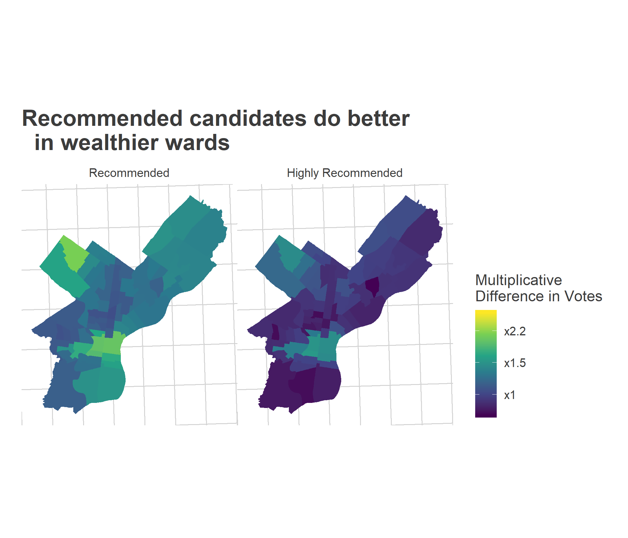
What’s going on in the other wards? The Democratic Party is especially important, especially in the traditionally-strong Black wards. (Note, I can’t identify here if that’s because they strongly adopt the party’s endorsement, or if the party endorses the candidates who would already do well). Interestingly, the party wasn’t so important in the Hispanic wards of North Philly or the Northeast.
View code
ggplot(
ward_effects %>%
filter(variable_name %in% c(format_variables[3]))
) +
geom_sf(aes(fill=effect), color = NA) +
facet_wrap(~variable_name) +
scale_fill_viridis_c(
"Multiplicative\nDifference in Votes",
labels=format_effect,
breaks = seq(-2, 3, 0.4)
) +
theme_map_sixtysix() %+replace%
theme(legend.position="right") +
expand_limits(fill = fill_min) +
ggtitle("Party-endorsed candidates\ndo better in predominantly-Black wards")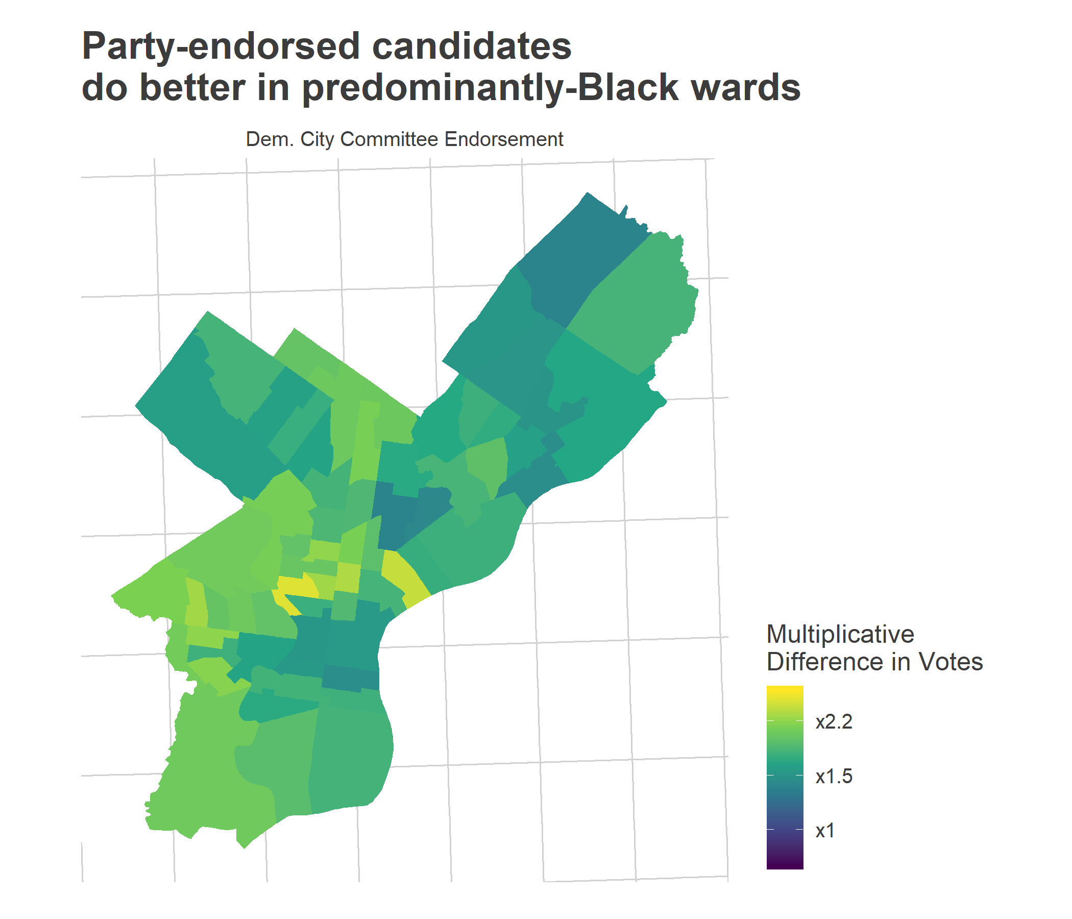
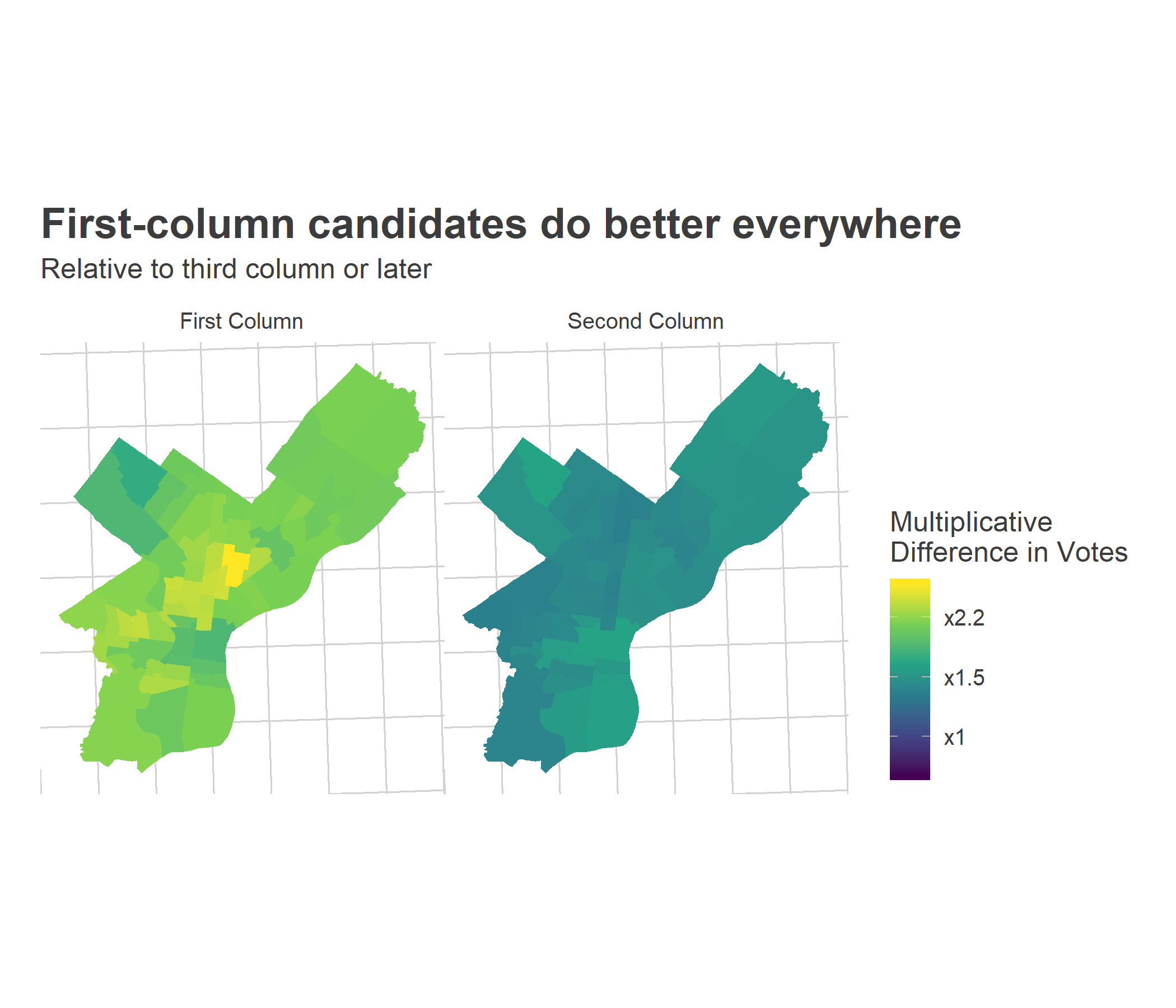
Unfortunately, all of these effects are swamped by ballot position. Candidates in the first column receive twice as many votes in every single type of ward, but especially many in lower-income wards.
View code
ggplot(
ward_effects %>%
filter(variable_name %in% c(format_variables[4:5]))
) +
geom_sf(aes(fill=effect), color = NA) +
facet_wrap(~variable_name) +
scale_fill_viridis_c(
"Multiplicative\nDifference in Votes",
labels=format_effect,
breaks = seq(-2, 3, 0.4)
) +
theme_map_sixtysix() %+replace%
theme(legend.position="right") +
expand_limits(fill = fill_min) +
ggtitle(
"First-column candidates do better everywhere",
"Relative to third column or later"
)
Simulating the election
The task of predicting the election comes down to using these correlations, and then randomly sampling uncertainty of the correct size.
I use each candidate’s ballot position and endorsements to come up with a baseline estimate of how they’ll do in each ward. There is a lot of uncertainty for a given candidate, so I add random noise to each candidate (candidate-level effects that aren’t explained by my model have a standard deviation of about +/- 30% of their votes.)
I scale up the ward performance by my turnout projection. I’m using my high-turnout projections, which assume that the post-2016 surge continues in Center City and its ring, and will in general help recommended candidates, who do better in those wealthier wards.
View code
turnout_2019 <- read.csv(
"../turnout_2019_primary/turnout_projections_2019.csv"
) %>%
mutate(WARD = sprintf("%02d", WARD16)) %>%
group_by(WARD) %>%
summarise(
high_projection = sum(high_projection, na.rm = TRUE),
low_projection = sum(low_projection, na.rm = TRUE)
)

replace_na <- function(x, r=0) ifelse(is.na(x), r, x)

df_2019 <- ballot %>%
filter(year == 2019) %>%
mutate(
philacommrec = replace_na(philacommrec),
dcc = replace_na(dcc),
inq = (philacommrec > 0),
year = 2017  ## fake year to trick lm
) %>%
prep_df_for_lm(use_candidate = FALSE) %>%
left_join(
expand.grid(
name = unique(ballot$name),
WARD = unique(turnout_2019$WARD)
)
) %>% left_join(turnout_2019)


## pretend it's one candidate, but then marginalize over candidates
df_2019$log_pvote <- predict(
rfit,
newdata = df_2019 %>%
mutate(candidate_year = df_complemented$candidate_year[1])
)

df_2019 <- df_2019 %>%
mutate(pvote_prop = exp(log_pvote))

sd_cand <- sd(ranef(rfit)$candidate_year$`(Intercept)`)
simdf <- expand.grid(
sim = 1:1000,
name = unique(df_2019$name)
) %>%
mutate(cand_re = rnorm(n(), sd = sd_cand))

## https://econsultsolutions.com/simulating-the-court-of-common-pleas-election/
votes_per_voter <- 4.5

simdf <- df_2019 %>%
left_join(simdf) %>%
mutate(pvote_prop_sim = pvote_prop * exp(cand_re)) %>%
group_by(WARD, sim) %>%
mutate(pvote = pvote_prop_sim / sum(pvote_prop_sim)) %>%
group_by() %>%
mutate(votes = high_projection * votes_per_voter * pvote) %>%
group_by(sim, name) %>%
summarise(votes = sum(votes)) %>%
left_join(ballot %>% filter(year == 2019)) %>%
prep_df_for_lm(use_candidate = FALSE)

simdf <- simdf %>%
group_by(sim) %>%
mutate(
vote_rank = rank(desc(votes)),
winner = rank(vote_rank) <= 6
)

remove_na <- function(x, r=0) return(ifelse(is.na(x), r, x))

winner_df <- simdf %>%
group_by(sim) %>%
summarise(
winners_rec = sum(is_rec * winner),
winners_highly_rec = sum(is_highly_rec * winner),
winners_col1 = sum(col1 * winner),
winners_col2 = sum(col2 * winner),
winners_col3 = sum(col3 * winner),
winners_dcc = sum(remove_na(dcc) * winner),
winners_women = sum((gender == "F") * winner)
)
Under the hood, the model has an estimate for each candidate. But I’m not totally comfortable with blasting those out (and what feedback loops that might cause), so let’s look at the high-level predictions instead.
View code
col_sim <- winner_df %>%
select(winners_col1, winners_col2) %>%
mutate(
`Third Column or later` = 6 - winners_col1 - winners_col2
) %>%
rename(
`First Column` = winners_col1,
`Second Column` = winners_col2
)

rec_sim <- winner_df %>%
select(winners_rec, winners_highly_rec, winners_dcc) %>%
mutate(
`Not Recommended` = 6 - winners_rec
) %>%
rename(
`All Recommended` = winners_rec,
`Highly Recommended` = winners_highly_rec,
`DCC Endorsed` = winners_dcc
)

gender_sim <- winner_df %>%
select(winners_women) %>%
mutate(
`Men` = 6 - winners_women
) %>%
rename(
`Women` = winners_women
)

plot_winners <- function(
sim_df,
title,
facet_order,
colors
){
gathered_df <- sim_df %>%
gather("facet", "n_winners") %>%
mutate(
facet = factor(
facet,
facet_order
)
) %>%
group_by(facet, n_winners) %>%
count() %>%
group_by(facet) %>%
mutate(prop = n / sum(n))

facet_lev <- levels(gathered_df$facet)
names(colors) <- facet_lev
ggplot(
gathered_df,
aes(x=n_winners)
) +
geom_bar(aes(y = prop, fill = facet), stat="identity") +
theme_sixtysix() +
expand_limits(x=c(0,7)) +
scale_x_continuous("Count of winners", breaks = 0:7) +
ylab("Proportion of simulations") +
scale_fill_manual(values = colors, guide=FALSE)+
facet_grid(facet~.) +
geom_vline(xintercept=6, linetype="dashed") +
ggtitle(title)
}
The model is really optimistic about how many Recommended candidates win, mostly because there’s only one Not Recommended candidate in the first two columns. In 66% of simulations all six winners are Recommended, and in 33% all but one are (Jon Marshall at the bottom of the first column is usually the lone Not Recommended winner).
View code
plot_winners(
rec_sim,
"Simulations by Recommendation",
c("Highly Recommended", "All Recommended", "Not Recommended", "DCC Endorsed"),
c(strong_blue, strong_green, strong_red, strong_grey)
)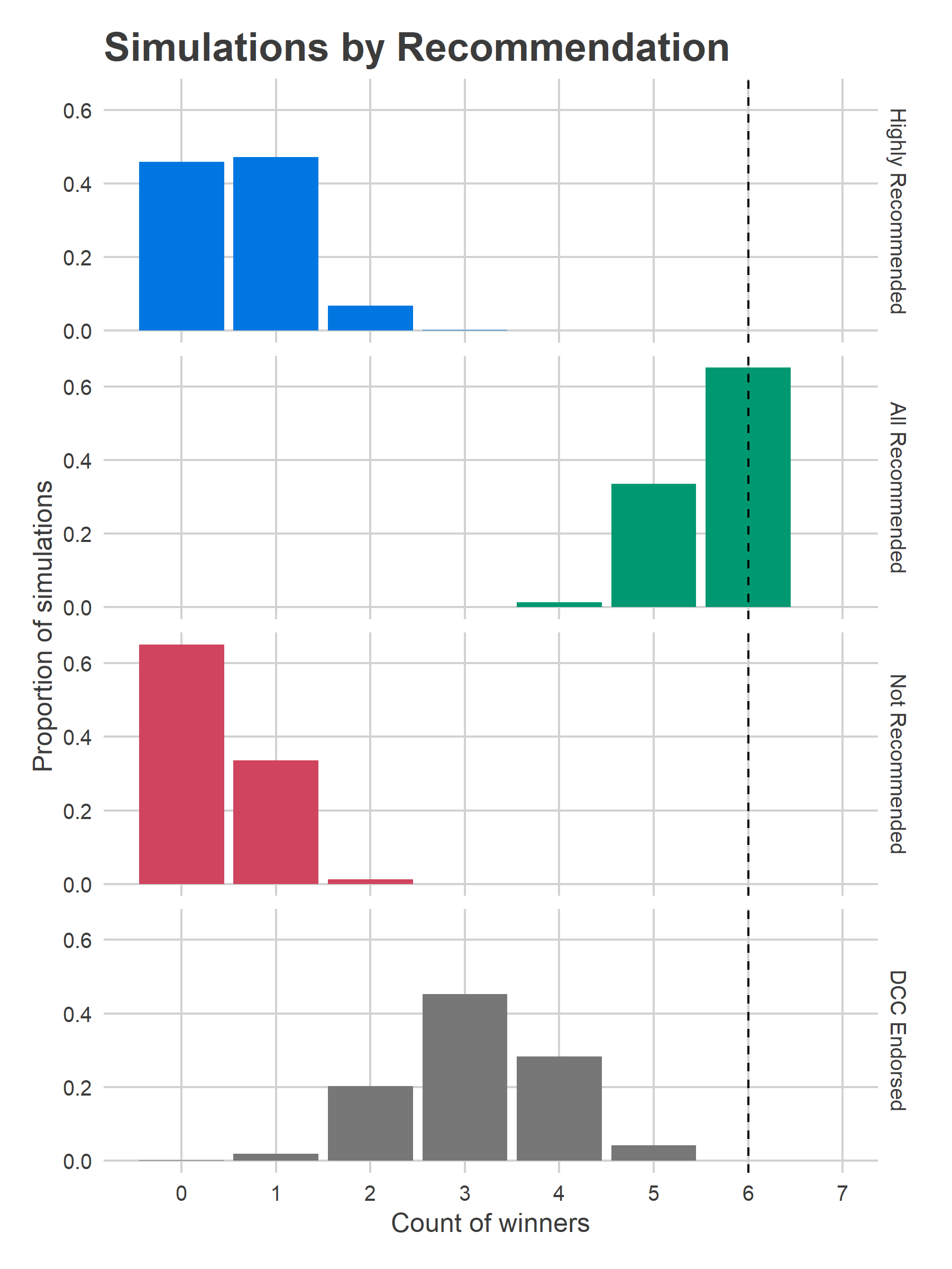
Highly Recommended candidates do less well; we get no Highly Recommended winners in 46% of simulations, and only one in another 47%. Remember that the model doesn’t think that being Highly Recommended helps more than just regular Recommended, and this year’s candidates have bad ballot position. Their performance this year will be a barometer for the power of the Bar’s endorsements; getting two winners (let alone three or four) would be a huge achievement (and presumably good for the citizens of Philadelphia, too).
DCC endorsees win an average of 3.1 of the six seats.
Of course, the true determinant is the first column.
View code
plot_winners(
col_sim,
"Simulations by Column Position",
c("First Column", "Second Column", "Third Column or later"),
c(strong_purple, strong_orange, strong_grey)
)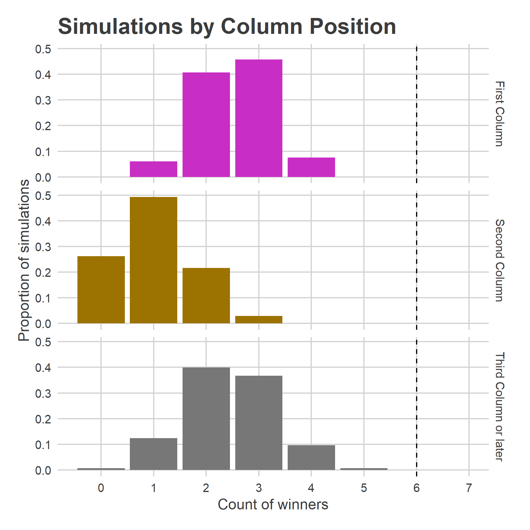
The first column produces 2.5 winners on average; the most likely outcome is three of the first-column candidates winning (45% of simulations), the second most likely is two (40%). The second column still produces 1.0 winners on average, with the remaining 2.4 winners coming from the final five columns.
View code
wincount_df <- simdf %>%
group_by(sim) %>%
mutate(pvote= votes/sum(votes)) %>%
filter(vote_rank == 6)
How many votes will it take to win? The average sixth-place winner wins 5.1% of the vote (remember that candidates can vote for multiple candidates). Assuming that 218,000 people vote, and an average of 4.5 candidates selected per voter, that comes out to 50,000 votes.
View code
ggplot(
wincount_df,
aes(x = pvote * 100)
) +
geom_histogram(
aes(y=stat(count) / sum(stat(count))),
boundary=5,
binwidth=0.2,
fill = strong_green
) +
ylab("Proportion of Simulations") +
xlab("Percent of vote received by sixth place") +
geom_vline(xintercept = 100 * mean(wincount_df$pvote), color = "black") +
annotate(
"text",
label = sprintf("Mean = %.1f %%", 100 * mean(wincount_df$pvote)),
x = 100 * mean(wincount_df$pvote),
y = 0.05,
angle = 90,
vjust = 1.1
)+
theme_sixtysix() +
ggtitle("Win Count for Common Pleas") 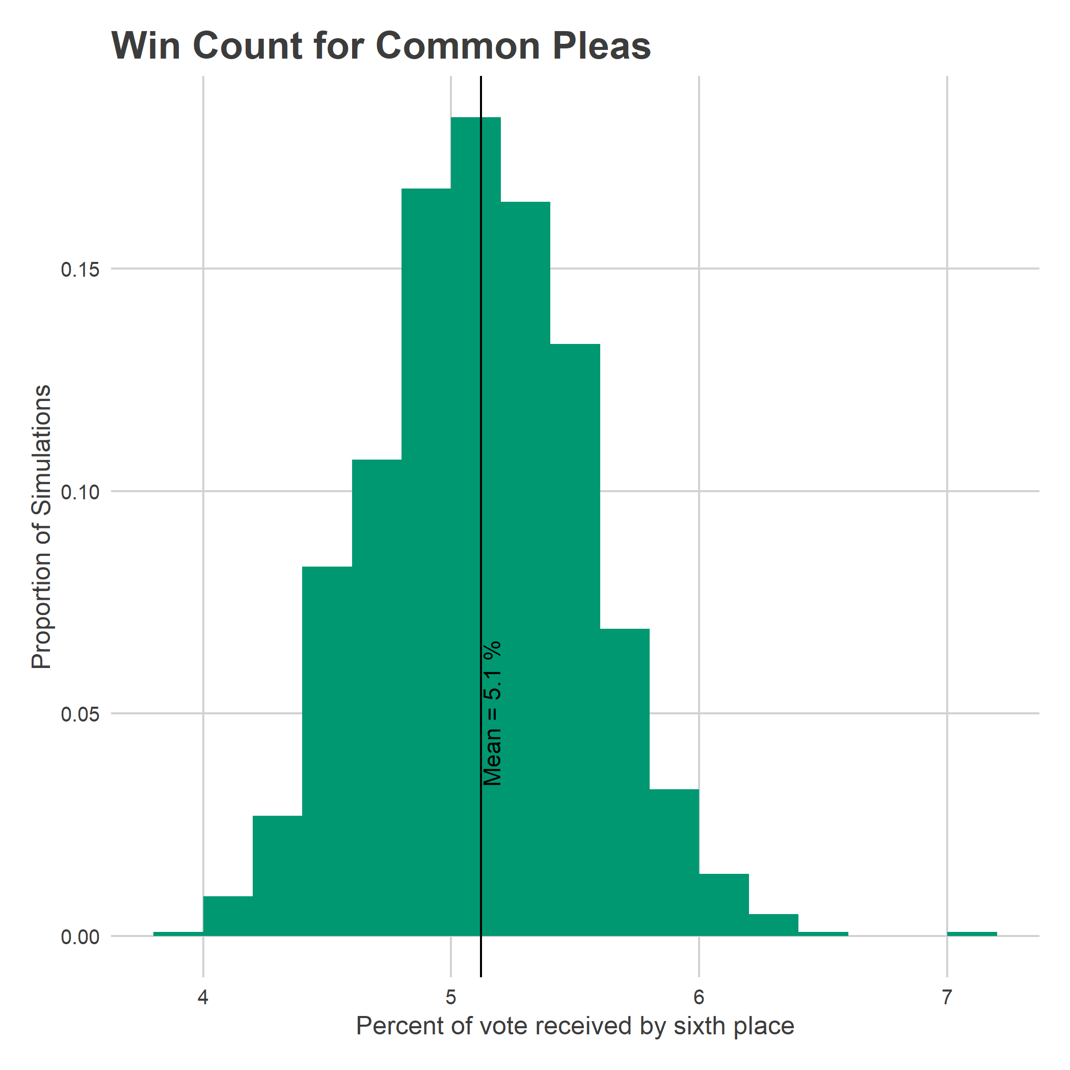
This year may be… not too bad?
In 2015, three Not Recommended candidates became ten year judges. In 2017, three more did. This year, probably at worst only one will. Why? Mostly luck; all six of those unqualified winners were in the first column, and this year seven of the eight candidates in the first two columns are Recommended.
Instead, the open question is just how qualified our judges will be. Will we stay on par with the past, which would see my model’s predicted zero or only one Highly Recommended candidate win? Or will the Bar’s Highly Recommended ratings assert themselves, and prove a bigger player this year?
This write-up on the judicial race is excellent, as always. I notice that you factor in gender – why do females have an advantage? Also, how big of a boost do they get?
Good question! I may go back and add that in.
Women receive about 16% more votes, all else being equal. Presumably there is a chunk of the electorate that votes an all-female ballot.