In 2017, about 6 points
With ballot positions decided, candidates are starting to vie for coveted ward endorsements. How many votes are they really worth?
Two years ago, I did a simplistic analysis of the Court of Common Pleas, where I found that judicial candidates received 0.9 more percent of the vote in wards where they were endorsed. In a race where candidates win with 4.3 percent of the vote, that effect is huge (and larger than even ballot position).
There were a number of caveats to that analysis: I only had endorsements from a few, systematically different wards, and I didn’t do anything to identify causality–we know that candidates do better in wards where they are endorsed, but we don’t know if the endorsements cause that increase, or if the ward leaders were endorsing candidates who would have done well there anyway.
Let’s do better.
In 2017, Max Marin at Philadelphia Weekly undertook the herculean effort of tracking down endorsements in 62 of Philadelphia’s 66 wards. Let’s use that, and do some spatial econometrics.
View code
library(tidyverse)
library(sp)
library(rgeos)
library(rgdal)
library(sf)
source("../../admin_scripts/util.R")

df_major <- safe_load("../../data/processed_data/df_major_2017_12_01.Rda")

df_major$WARD_DIVSN <- with(df_major, paste0(WARD16, DIV16))

df_major <- df_major %>%
  filter(
    election == "primary" & CANDIDATE != "Write In" & PARTY == "DEMOCRATIC"
  )
df_major <- df_major %>%
  group_by(WARD_DIVSN, OFFICE, year) %>%
  mutate(pct_vote = VOTES / sum(VOTES))

df_major <- df_major %>%
  filter(OFFICE %in% c("COUNCIL AT LARGE", "DISTRICT ATTORNEY"))


bg_17_acs <- read.csv("../../data/census/acs_2013_2017_phila_bg_race_income.csv")
bg_17_acs <- bg_17_acs %>%
  mutate(Geo_FIPS = as.character(Geo_FIPS)) %>%
  select(
    Geo_FIPS, pop, pop_nh_white, pop_nh_black, pop_nh_asian, pop_hisp, pop_median_income_2017
  )

sp_divs <- readOGR("../../data/gis/2016/2016_Ward_Divisions.shp", verbose = FALSE)
sp_divs <- spChFIDs(sp_divs, as.character(sp_divs$WARD_DIVSN))
sp_divs <- spTransform(sp_divs, CRS("+init=EPSG:4326"))

library(tigris)
options(tigris_use_cache = TRUE)
bg_shp <- block_groups(42, 101, year = 2015)
bg_shp <- spChFIDs(bg_shp, as.character(bg_shp$GEOID))
bg_shp <- spTransform(bg_shp, CRS(proj4string(sp_divs)))

sp_divs$bg <- over(
  gCentroid(sp_divs, byid = TRUE),
  bg_shp
)$GEOID

sp_divs@data <- sp_divs@data %>%
  left_join(bg_17_acs, by = c("bg"="Geo_FIPS"))

df_major <- df_major %>%
  left_join(sp_divs@data) %>%
  mutate(
    pct_wht = pop_nh_white / pop,
    pct_blk = pop_nh_black / pop,
    pct_asian = pop_nh_asian/ pop,
    pct_hisp = pop_hisp / pop
  )
In the 2017 DA race, no single candidate monopolized the endorsements; O’Neill led the way with 11 endorsements, largely in the Northeast.
View code
endorsements <- read_csv("da_2017_endorsements.csv")
endorsements$ward <- sprintf("%02d", endorsements$ward)

da_results <- df_major %>%
  filter(election == "primary" & year == 2017 & OFFICE == "DISTRICT ATTORNEY") %>%
  mutate(
    last_name = gsub(
      "^.*\\s([A-Z])([A-Z]+)
View code
quot;, "\\U\\1\\L\\2", CANDIDATE, perl = TRUE ) ) %>% group_by(WARD_DIVSN) %>% mutate(total_votes = sum(VOTES)) %>% group_by() %>% mutate(pvote = VOTES / total_votes) da_results$last_name <- with( da_results, ifelse( last_name == "Neill", "O'Neill", ifelse(last_name == "Shabazz", "El-Shabazz", last_name) ) ) da_results %>% group_by(WARD16, last_name) %>% summarise(votes = sum(VOTES)) %>% group_by(WARD16) %>% mutate( ward_votes = sum(votes), pvote = votes/ ward_votes ) %>% left_join( endorsements %>% mutate(is_endorsed = TRUE), by = c("WARD16" = "ward", "last_name" = "endorsement") ) %>% mutate( is_endorsed = replace(is_endorsed, is.na(is_endorsed), FALSE) ) %>% group_by(last_name, is_endorsed) %>% summarise( pct_vote = 100 * weighted.mean(pvote, w = ward_votes), total_votes = sum(ward_votes), n_wards = n() ) %>% group_by(last_name) %>% summarise( pct_vote_overall = weighted.mean(pct_vote, w = total_votes), wards_endorsed = ifelse(any(is_endorsed), n_wards[is_endorsed], 0), turnout_endorsed = ifelse(any(is_endorsed), total_votes[is_endorsed], 0), pct_vote_notendorsed = pct_vote[!is_endorsed], pct_vote_endorsed = ifelse(any(is_endorsed), pct_vote[is_endorsed], NA) ) %>% arrange(desc(pct_vote_overall)) %>% knitr::kable( digits = 0, format = "html", format.args = list(big.mark = ","), col.names = c( "Candidate", "Citywide % of vote", "Number of ward endorsements", "Turnout in endorsed wards", "% of vote in un-endorsed wards", "% of vote in endorsed wards" ) )
| Candidate | Citywide % of vote | Number of ward endorsements | Turnout in endorsed wards | % of vote in un-endorsed wards | % of vote in endorsed wards |
|---|---|---|---|---|---|
| Krasner | 38 | 9 | 28,700 | 36 | 46 |
| Khan | 20 | 8 | 23,485 | 18 | 32 |
| Negrin | 14 | 10 | 20,794 | 13 | 21 |
| El-Shabazz | 12 | 7 | 19,504 | 11 | 17 |
| Untermeyer | 8 | 9 | 16,200 | 7 | 17 |
| O’Neill | 6 | 11 | 21,520 | 4 | 20 |
| Deni | 2 | 0 | 0 | 2 | NA |
Krasner won by over 5,000 votes (18%), despite receiving the typical number of ward endorsements. The endorsements that he did receive came from wards with the highest turnout, but part of that is reverse causality: the places that he energized turned out big.
Naively, candidates did about 11 percentage points better in wards where they were endorsed than in wards where they weren’t. BUT. This suffers from the same lack of causal identification as the Judicial Analysis above: we don’t know if they did better because of the endorsements, or if they were just endorsed in wards where they would have done well anyway.
How can we do better? Let’s use something I noticed in last week’s post on District 7: the strength of boundaries.
The strongest ward endorsements can have visible effects in divisions just across the street from each other.
View code
wards <- readOGR("../../data/gis/2016","2016_Wards", verbose=FALSE) %>%
spTransform(CRS(proj4string(sp_divs)))
ggwards <- fortify(spChFIDs(wards, sprintf("%02d", wards$WARD)))
bbox <- sp_divs[substr(sp_divs$WARD_DIVSN,1,2) %in% c("10", "50", "09"),] %>%
gUnionCascaded() %>%
bbox()
bbox <- rowMeans(bbox) + 1.2 * sweep(bbox, 1, rowMeans(bbox))
polygon_in_bbox <- function(p) {
coords <- p@Polygons[[1]]@coords
any(
coords[,1] > bbox[1,1] &
coords[,1] < bbox[1,2] &
coords[,2] > bbox[2,1] &
coords[,2] < bbox[2,2]
)
}
sp_divs$in_bbox <- sapply(sp_divs@polygons, polygon_in_bbox)
ggdivs <- fortify(spChFIDs(sp_divs, as.character(sp_divs$WARD_DIVSN)))
ggdivs <- ggdivs %>%
left_join(
sp_divs@data %>% select(WARD_DIVSN, in_bbox),
by = c("id" = "WARD_DIVSN")
) %>%
left_join(
da_results %>% filter(last_name %in% c("Khan", "Krasner", "El-Shabazz")),
by = c("id" = "WARD_DIVSN")
)
ward_centroids <- gCentroid(wards, byid=TRUE) %>% as.data.frame()
ward_centroids$ward <- wards$WARD
ggplot(
ggdivs %>% filter(in_bbox),
aes(x=long, y=lat)
) +
geom_polygon(aes(fill = 100 * pvote, group=group), color = NA) +
geom_polygon(data = ggwards, aes(group=group), fill = NA, color = "white") +
geom_text(data = ward_centroids, aes(x=x, y=y, label=ward), color = "white") +
facet_wrap(~last_name) +
scale_fill_viridis_c("% of vote") +
theme_map_sixtysix() +
coord_map(xlim=bbox[1,], ylim=bbox[2,]) +
theme(
legend.position = "bottom",
legend.direction = "horizontal"
) +
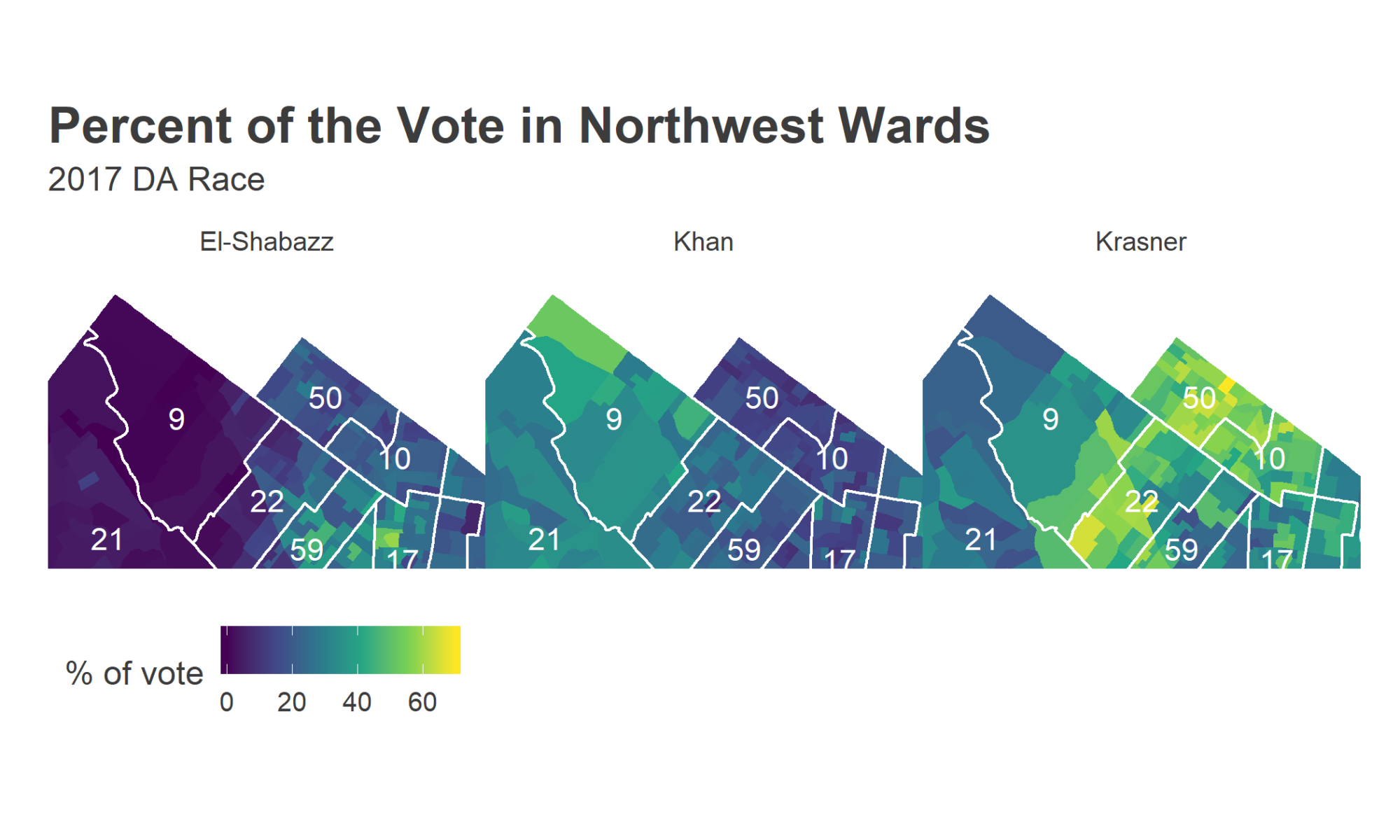
ggtitle("Percent of the Vote in Northwest Wards", "2017 DA Race")
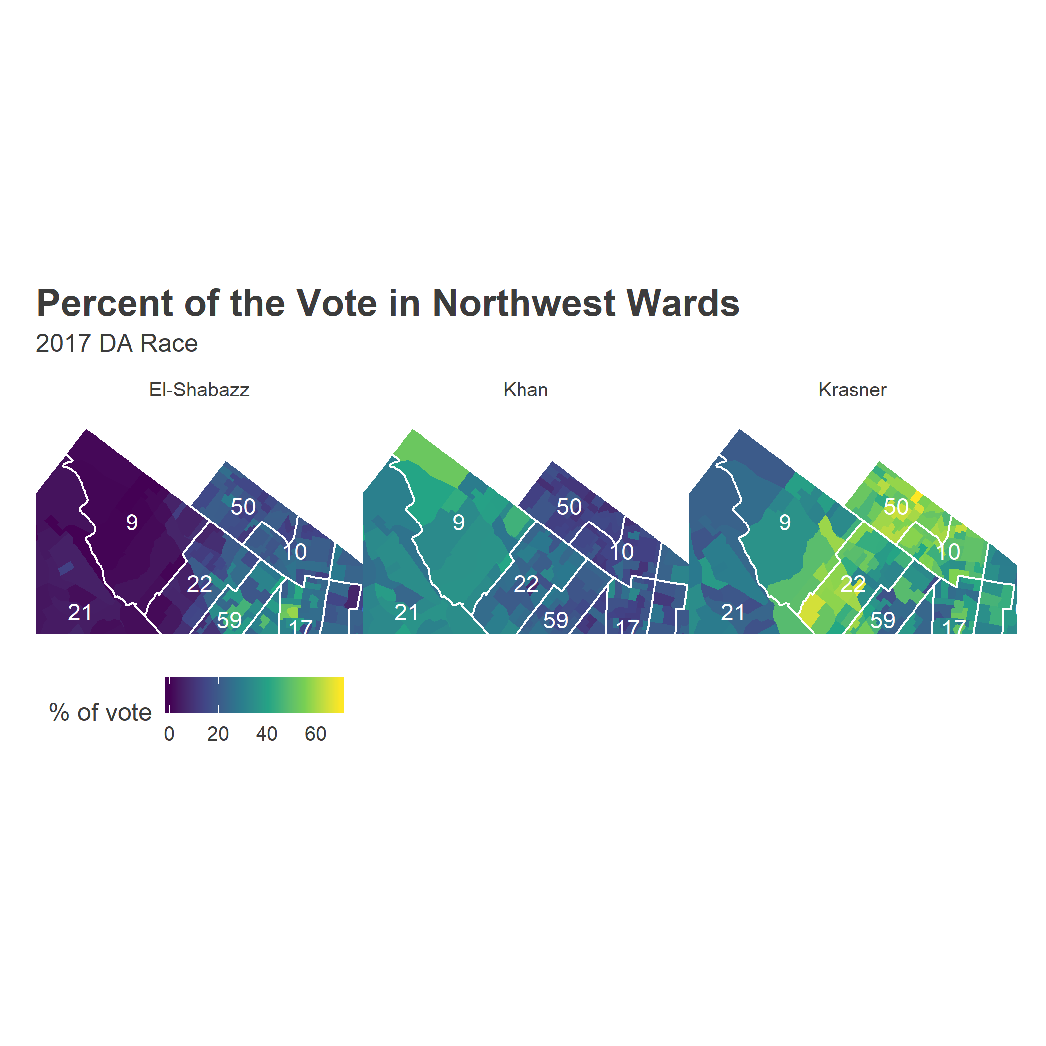
Wards 10 and 50 endorsed Krasner, Ward 9 endorsed Khan, and Ward 22 endorsed El-Shabazz. You can immediately see the strength of 10 and 50’s endorsements: Krasner did better in divisions inside the boundary of 10 and 50 than he did just across the street. Same for 9, maybe, where Khan did well. And El-Shabazz did better in 22, though there isn’t an obvious boundary effect.
I’ll use this intuition to measure the effect across all boundaries in the whole city. To isolate the causal effect of the wards, I’ll limit the analysis to only compare divisions that are across the street from each other but happen to be divided by a ward boundary, and where different candidates were endorsed. This will ensure that we’re comparing divisions apples-to-apples, where the only thing that’s different is the ward endorsement.
I’ll go one step farther, and control for the census demographics of the block groups that the division sits in, in case a ward boundary happens to also serve as an emergent boundary (dissertation plug). I measure how each candidate’s vote correlated with the race and ethnicity of the neighborhood and subtract that out, leaving a measure of how much better or worse that candidate did than expected. It’s that “residual” that I will compare across boundaries.
View code
da_fit <- lm(
  pvote ~
    CANDIDATE * pct_wht +
    CANDIDATE * pct_blk +
    CANDIDATE * pct_hisp,
    # CANDIDATE * log(pop_median_income_2017),
  data = da_results
)

da_results$predicted <- predict(da_fit, newdata = da_results)
da_results$resid <- with(da_results, pvote - predicted)

neighbors <- st_intersection(st_as_sf(sp_divs), st_as_sf(sp_divs))
neighbors <- neighbors %>%
  filter(WARD != WARD.1)

neighbors <- neighbors %>%
  mutate(geometry_type = st_geometry_type(geometry)) %>%
  filter(!geometry_type %in% c("POINT", "MULTIPOINT"))


neighbors <- neighbors %>%
  mutate(
    WARD.0 = sprintf("%02d", asnum(WARD)),
    WARD.1 = sprintf("%02d", asnum(WARD.1))
  ) %>%
  left_join(
    endorsements %>% rename(endorsement.0 = endorsement),
    by = c("WARD.0" = "ward")
  ) %>%
  left_join(
    endorsements %>% rename(endorsement.1 = endorsement),
    by = c("WARD.1" = "ward")
  )

neighbors <- neighbors %>%
  left_join(
    da_results %>%
      select(WARD_DIVSN, last_name, total_votes, pvote, resid) %>%
      rename(total_votes.0 = total_votes, pvote.0 = pvote, resid.0 = resid),
    by = c("WARD_DIVSN" = "WARD_DIVSN", "endorsement.0" = "last_name")
  ) %>%
  left_join(
    da_results %>%
      select(WARD_DIVSN, last_name, total_votes, pvote, resid) %>%
      rename(total_votes.1 = total_votes, pvote.1 = pvote, resid.1 = resid),
    by = c("WARD_DIVSN.1" = "WARD_DIVSN", "endorsement.0" = "last_name")
  )
To correctly measure wards’ individual strength, I fit a random effects model, which simultaneously estimates the average effect of all wards’ endorsements and how much each individual ward varies from that.
View code
library(lme4)

df0 <- neighbors %>% filter(endorsement.0 != endorsement.1)

fit_lmer <- function(neighbor_df){
  re_fit <- lmer(
    resid.0 - resid.1 ~ (1 | WARD.0),
    data = neighbor_df,
    weights = neighbor_df %>%
      with(pmin(total_votes.0, total_votes.1))
  )

  re <- ranef(re_fit)$WARD.0
  re <- re %>%
    mutate(
      ward = row.names(re),
      effect = re_fit@beta + `(Intercept)`
    )

  return(
    list(
      fit = re_fit,
      re = re
    )
  )
}

fit_baseline <- fit_lmer(df0)

n_boot <- 200
bs_list <- vector(mode = "list", length = n_boot)
for(b in 1:n_boot){

  sample_divs = sample(unique(df0$WARD_DIVSN), replace = TRUE)

  #if(b %% floor(n_boot / 10) == 0) print(b)
  df_samp <- data.frame(WARD_DIVSN = sample_divs) %>% left_join(df0)
  bs_fit <- fit_lmer(df_samp)
  bs_list[[b]] <- bs_fit
}

fixef_ci <- quantile(
  sapply(bs_list, function(x) fixef(x$fit)),
  c(0.025, 0.975)
)
cat(paste0(
  "Average Effect of a Ward Endorsement:\n",
  sprintf(
    "%0.1f (%0.1f, %0.1f)",
    fixef(fit_baseline$fit)["(Intercept)"] * 100,
    fixef_ci[1] * 100,
    fixef_ci[2] * 100
  )
))
## Average Effect of a Ward Endorsement:
## 5.8 (5.0, 6.9)
The average Ward endorsement was worth 5.8 percentage points in the 2017 DA race. This is about half of the 11 percentage point gap we saw in the naive analysis above; it turns out the other half was because of wards endorsing candidates that the voters already supported.
But some wards are much more important than others.
How does each ward’s endorsement stack up? The table below sorts the wards by order of the vote effect, which is the percentage effect of the endorsement times the 2017 primary turnout.
View code
ranef_ci <- bind_rows(
  lapply(bs_list, function(x) x$re),
  .id = "sim"
) %>%
  group_by(ward) %>%
  summarise(
    p025 = quantile(effect, 0.025),
    p975 = quantile(effect, 0.975)
  )

fit_baseline$re %>%
  select(ward, effect) %>%
  left_join(ranef_ci) %>%
  mutate(
    ci = sprintf("(%0.1f, %0.1f)", 100 * p025, 100*p975)
  ) %>%
  left_join(
    da_results %>%
      group_by(WARD16, last_name) %>%
      summarise(
        pvote = 100 * weighted.mean(pvote, w = total_votes),
        total_votes = sum(total_votes)
      ) %>%
      inner_join(
        endorsements,
        by = c("WARD16" = "ward", "last_name" = "endorsement")
      ),
    by = c("ward" = "WARD16")
  ) %>%
  mutate(
    pvote = round(pvote, 0),
    effect = round(100 * effect, 0),
    vote_effect = round(effect/100 * total_votes)
  ) %>%
  rename(endorsement = last_name) %>%
  select(ward, endorsement, pvote, effect, ci, total_votes, vote_effect) %>%
  arrange(desc(vote_effect)) %>%
  DT::datatable(
    rownames=FALSE,
    colnames = c("Ward", "Endorsee", "% of Vote in Ward", "Endorsement Effect at Boundary","CI", "Ward Votes", "Vote Effect of Endorsement")
  )
| Ward | Endorsee | % of Vote in Ward | Endorsement Effect at Boundary | CI | Ward Votes | Vote Effect of Endorsement |
|---|---|---|---|---|---|---|
| 10 | Krasner | 50 | 14 | (8.0, 19.5) | 3,719 | 521 |
| 09 | Khan | 37 | 12 | (6.7, 17.5) | 4,264 | 512 |
| 30 | Khan | 39 | 14 | (8.5, 17.9) | 3,403 | 476 |
| 52 | Negrin | 17 | 10 | (1.1, 20.0) | 3,768 | 377 |
| 36 | Negrin | 18 | 9 | (4.8, 13.6) | 3,932 | 354 |
| 56 | Untermeyer | 26 | 14 | (9.9, 19.5) | 2,346 | 328 |
| 50 | Krasner | 56 | 6 | (-0.7, 15.6) | 5,094 | 306 |
| 61 | El-Shabazz | 24 | 12 | (4.7, 19.3) | 2,547 | 306 |
| 40 | O’Neill | 15 | 8 | (4.8, 14.3) | 3,591 | 287 |
| 42 | Krasner | 45 | 20 | (14.6, 25.2) | 1,270 | 254 |
| 38 | Negrin | 29 | 10 | (3.3, 21.0) | 2,507 | 251 |
| 01 | O’Neill | 13 | 7 | (3.7, 9.1) | 2,954 | 207 |
| 03 | Untermeyer | 22 | 8 | (3.0, 14.3) | 2,312 | 185 |
| 63 | O’Neill | 24 | 8 | (2.4, 16.0) | 1,920 | 154 |
| 19 | Negrin | 50 | 26 | (16.4, 40.6) | 589 | 153 |
| 57 | O’Neill | 26 | 8 | (4.5, 13.0) | 1,719 | 138 |
| 65 | O’Neill | 26 | 8 | (5.9, 11.0) | 1,644 | 132 |
| 23 | O’Neill | 20 | 10 | (5.2, 18.7) | 1,284 | 128 |
| 05 | Khan | 30 | 2 | (-2.5, 7.2) | 5,927 | 119 |
| 60 | Negrin | 15 | 5 | (2.0, 8.2) | 2,350 | 118 |
| 07 | Negrin | 55 | 21 | (6.2, 36.9) | 548 | 115 |
| 21 | Khan | 34 | 2 | (-3.3, 8.7) | 5,383 | 108 |
| 31 | Khan | 23 | 5 | (0.4, 9.0) | 2,076 | 104 |
| 24 | Untermeyer | 11 | 7 | (4.4, 11.0) | 1,437 | 101 |
| 51 | Untermeyer | 13 | 4 | (1.8, 9.8) | 2,386 | 95 |
| 46 | El-Shabazz | 9 | 2 | (-0.9, 5.3) | 4,515 | 90 |
| 16 | Untermeyer | 21 | 9 | (1.7, 13.0) | 965 | 87 |
| 12 | Krasner | 42 | 3 | (-0.7, 7.8) | 2,627 | 79 |
| 27 | Krasner | 70 | 4 | (-3.2, 11.4) | 1,978 | 79 |
| 41 | Khan | 24 | 7 | (3.9, 11.0) | 975 | 68 |
| 48 | Untermeyer | 13 | 4 | (1.8, 7.8) | 1,623 | 65 |
| 64 | O’Neill | 22 | 7 | (-0.8, 13.8) | 795 | 56 |
| 58 | Untermeyer | 15 | 2 | (-6.2, 7.2) | 2,606 | 52 |
| 14 | Negrin | 12 | 5 | (2.8, 7.9) | 986 | 49 |
| 34 | Krasner | 34 | 1 | (-3.6, 5.2) | 4,900 | 49 |
| 06 | Krasner | 47 | 3 | (-10.0, 10.1) | 1,605 | 48 |
| 39 | O’Neill | 25 | 1 | (-1.3, 5.9) | 4,462 | 45 |
| 43 | Negrin | 23 | 4 | (-0.1, 8.4) | 1,091 | 44 |
| 25 | Untermeyer | 14 | 5 | (-1.5, 11.7) | 801 | 40 |
| 55 | O’Neill | 18 | 3 | (-2.8, 7.9) | 1,305 | 39 |
| 54 | O’Neill | 11 | 4 | (0.8, 6.5) | 720 | 29 |
| 62 | O’Neill | 23 | 2 | (-1.8, 5.8) | 1,126 | 23 |
| 45 | Khan | 22 | 2 | (-1.6, 5.5) | 891 | 18 |
| 32 | El-Shabazz | 27 | 1 | (-3.3, 6.7) | 1,727 | 17 |
| 33 | Khan | 26 | 3 | (-1.4, 9.3) | 566 | 17 |
| 35 | Untermeyer | 11 | 1 | (-1.9, 5.6) | 1,724 | 17 |
| 04 | El-Shabazz | 31 | 0 | (-3.1, 4.5) | 2,110 | 0 |
| 44 | Krasner | 37 | 0 | (-5.4, 7.7) | 1,416 | 0 |
| 47 | El-Shabazz | 15 | -1 | (-5.0, 5.9) | 749 | -7 |
| 29 | Negrin | 23 | -2 | (-5.5, 4.2) | 1,331 | -27 |
| 15 | Negrin | 18 | -1 | (-5.1, 3.4) | 3,692 | -37 |
| 49 | El-Shabazz | 19 | -3 | (-7.1, 0.3) | 2,348 | -70 |
| 22 | El-Shabazz | 13 | -2 | (-4.5, 1.3) | 5,508 | -110 |
| 08 | Krasner | 42 | -3 | (-6.8, 0.6) | 6,091 | -183 |
The most important ward in 2017 was Ward 10, which gave Krasner a 14 percentage point boost on a turnout of 3,719, meaning an estimated bump of 507 votes. (The exact order of the rankings has a lot of uncertainty. Don’t take them as gospel.) Those three Northwest wards we looked at above, 10, 9 and 50, were all in the top seven, with 10 and 9 making up first and second place, largely on the back of their high turnout.
What this means for May
This analysis is specific to the 2017 DA race in a number of ways. I expect ward endorsements to have more importance in low-information races, and all of the races this time around–City Council At Large, Judicial, and Commissioner–will be lower-information than the 2017 DA.
Consider the simplistic analysis I did for the 2017 Court of Common Please. That analysis found that endorsed candidates performed 0.9 percentage points better, in a race that took 4.3% of the vote to win. That estimate is the analog to the 11 point DA effect in the first table. We found that half of the 11 DA points was actually causal, so 0.45 points is a naive guess of the effect in judicial races.
But there are two more changes. First, taking half of the effect is almost certainly too conservative for judges. There are few pre-existing preferences among voters, so much less of that correlation will be “wards endorsing candidates that are already popular”. The causal part will be higher.
But second, the wards that I had data for in that analysis are all the wards with the strongest endorsement effect in this one: 9, 30, 52, and 50 were all among the 18 wards I had data for. So that estimate might be higher, too, than if we had data for every ward.
We end up in between. The Ward endorsements–especially in the top wards on the chart–are effective but not decisive. They are powerful enough that they likely decide close judicial races, but not enough to have changed 2017’s DA race.
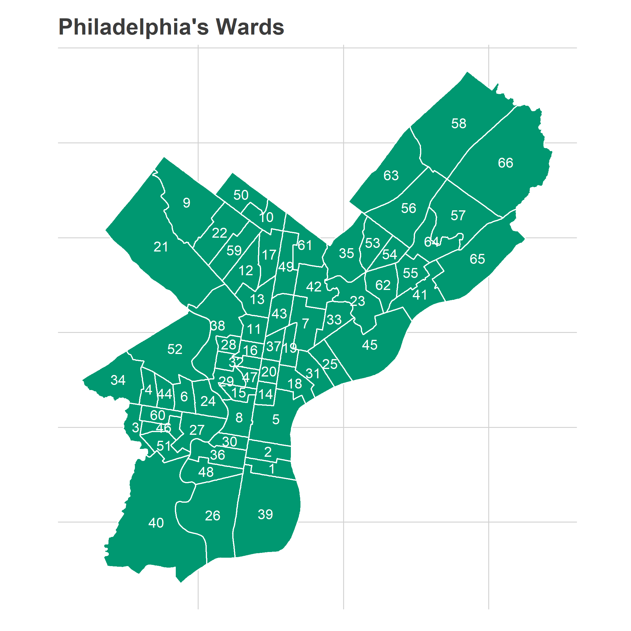
Appendix: Ward Map
View code
ggplot(ggwards, aes(x = long, y=lat)) +
  geom_polygon(aes(group=group), fill = strong_green, color = "white") +
  geom_text(data = ward_centroids, aes(x=x, y=y, label=ward), color = "white") +
  theme_map_sixtysix() +
  coord_map() +
  ggtitle("Philadelphia's Wards")
This is a great analysis! How is the ward endorsement information disseminated, and is it disseminated in the same way for each ward? For example, does each ward do a full-court press and send out one or more mailers highlighting its endorsement, along with having volunteers stand at the polls passing out an endorsement sheet? I would imagine that an endorsement gives a bigger boost if they spend more time/money/effort to get that information out as opposed to just telling a candidate “hey, you’re endorsed” and then doing nothing further. Also, do some wards do more to disseminate their endorsement to voters than others? I would guess that if a voter hasn’t been informed of who is endorsed by the time (s)he is in the voting booth, then that voter isn’t going to take the time to look that info up on his/her phone.
That’s absolutely crucial. The most effective wards are known for handing out sample ballots outside of each precinct, and even helping voters get to the polls. That’s almost certainly the difference. (check out https://phillyballots.tumblr.com/ for a sense of what they look like)