Tuesday is Election Day! Here’s how to participate with Sixty-Six Wards.
1. Vote!
2. Record your voter number, and submit it to https://bit.ly/sixtysixturnout
3. Follow along live at https://sixtysixwards.com/turnout-tracker/
4. Tell your friends!
Tuesday is Election Day! Here’s how to participate with Sixty-Six Wards.
1. Vote!
2. Record your voter number, and submit it to https://bit.ly/sixtysixturnout
3. Follow along live at https://sixtysixwards.com/turnout-tracker/
4. Tell your friends!
Last month, I saw a tweet from an Inquirer reporter celebrating the company’s win of the Newhouse School’s Toner Prize for Excellence in Local Reporting. I clicked through and saw the pieces for which it won. In a moment of frustration, I tweeted.

Enough people have asked me what this was about that I thought I’d write up a summary.
Clustering Philadelphia’s Elections
Back in 2019, I noticed that all of my maps of Philadelphia’s elections looked the same. Whether a map of turnout or the candidate that residents voted for, certain sections of the city moved together in each election. I ran a clustering algorithm on results from the prior eight Democratic Primaries, set to identify four clusters that I called Philadelphia’s “Voting Blocs,” and noted that these clusters were largely structured by race and class. I renamed them here, and used them to understand election results here, here, here, here, here, here, here, here, here, here, here, here, and here. In 2020, I measured how those clusters changed over time.
In February 2023, the Inquirer published an article running a clustering algorithm on the prior eight Democratic Primaries, set to identify six clusters. They noted that the clusters were largely structured by race and class. They later measured how those clusters changed over time.
The Inquirer’s work was well done, and their write-up significantly better than mine. The interactivity was neat. But the analytic strategy was the same, on the same data with the same takeaways. I reached out to the Inquirer asking that they cite my work in the article. I expected a short sentence saying “Jonathan Tannen has performed a similar analysis” buried at the bottom. Instead, they just said “no”.
The reasons for not citing my work that I received include, with my annotations in brackets:
Is the work different?
That last point is the only that would matter, if it were true. I admit that “different enough” can be a fuzzy distinction, and journalists (or bloggers) don’t follow the same citation practices as academics. Unfortunately, their analysis in no way passes even the most lenient definition of “different”.
Both pieces…
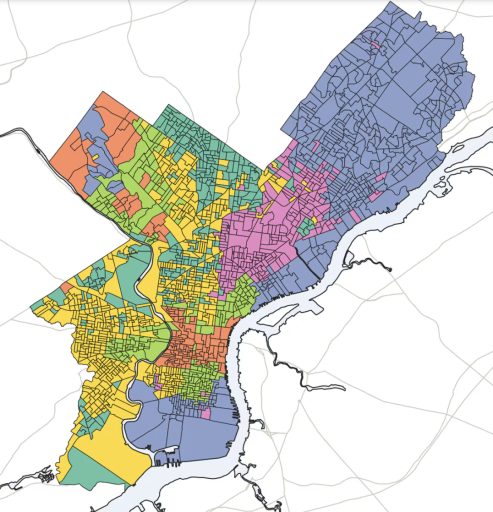
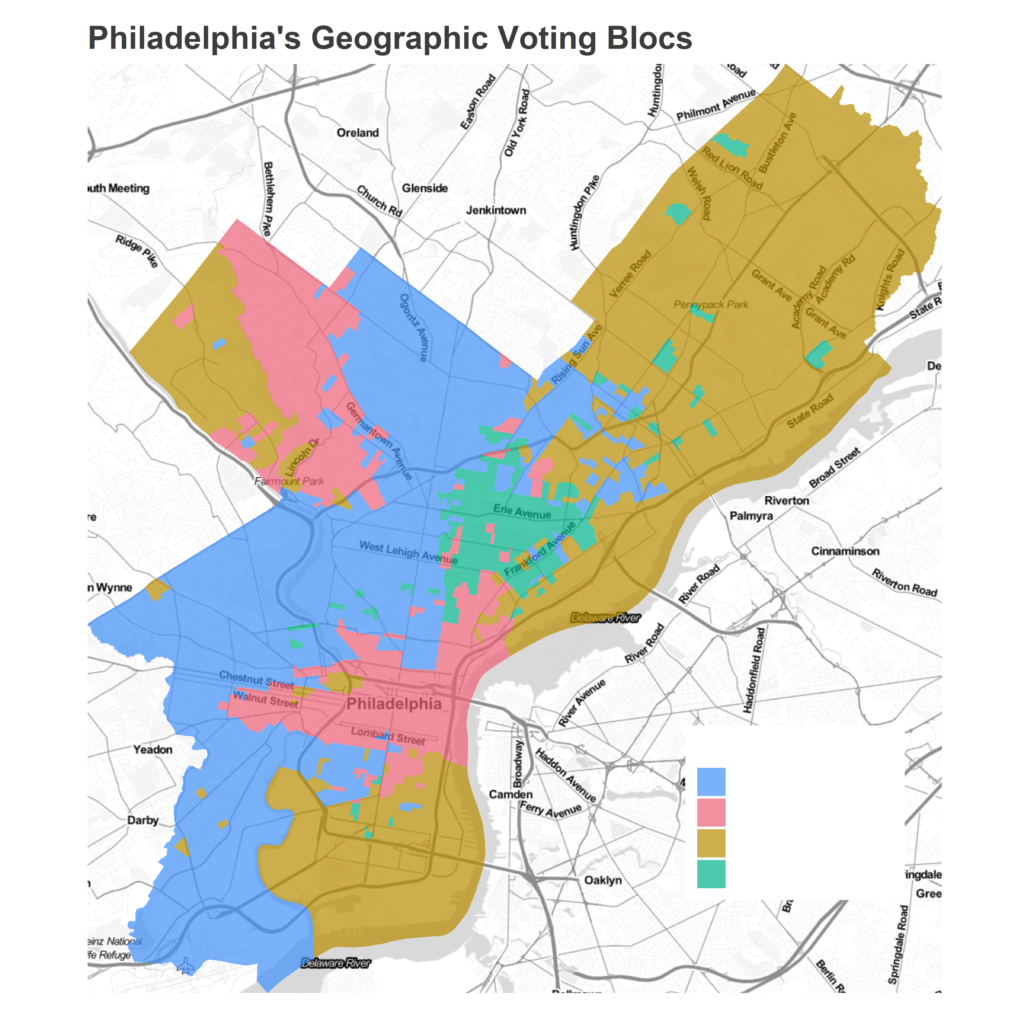
Here are the clusters they produced, and then mine.


You will notice, if you can see past color choice, that they are basically the same. The Inquirer divided my blue cluster into their yellow and dark green clusters, and divided my red cluster into their salmon and light green clusters. Maybe their pink cluster extends a few blocks north past my green one. But that’s it.
It’s hard to be sure of the differences under the hood, because unlike my blog the Inquirer has not published their code. But as far as I can tell, the only differences between the pieces are that (1) they ran it on 2013-2020 instead of 2012-2019 and (2) they set num_clusters=6 instead of num_clusters=4. Are those changes substantial? On their github page, the authors acknowledge “it’s worth noting that three-, four-, and five-cluster maps yielded similar results, and sussed out race and class boundaries in similar ways.”
In closing
I don’t know the inner workings of the Inquirer, so am hesitant to point fingers at the reporters of the piece. The authors did cite my work in the github branch that has five bookmarks. Of course, there’s a reason that I want my work to be cited in the article, and it’s the same reason that the Inquirer does not.
It’s brutal to watch the company celebrate an award for work that it plagiarized from mine. I hope that if the Inquirer continues to pursue “original” research, they will practice the bare minimum of citation requirements.