As the Mayor’s race heats up, I’m doing a series establishing some baseline numbers. What follows are simplistic calculations using reasonable assumptions. Welcome to the Back of the Envelope.
Breaking down the electorate
How many voters should we expect?
View code
library(tidyverse)
library(sf)

source("../../admin_scripts/util.R")


setwd("C:/Users/Jonathan Tannen/Dropbox/sixty_six/posts/council_ballot_position_23/")

df_major_type <- readRDS("../../data/processed_data/df_major_type_20230116.Rds")
df_major <- df_major_type %>%
  group_by(office, candidate, party, warddiv, year, election_type, district, ward, is_topline_office) %>%
  summarise(votes = sum(votes))

df_major <- df_major %>%
  group_by(year, election_type, office, district, warddiv) %>%
  mutate(pvote = votes / sum(votes)) %>%
  ungroup()

topline_votes <- df_major %>%
  filter(is_topline_office) %>%
  group_by(election_type, year) %>%
  summarise(votes = sum(votes)) %>%
  mutate(
    year = asnum(year),
    cycle = case_when(
      year %% 4 == 0 ~ "President",
      year %% 4 == 1 ~ "District Attorney",
      year %% 4 == 2 ~ "Governor",
      year %% 4 == 3 ~ "Mayor"
    )
  )

cycle_colors <- c("President" = strong_red, "Mayor" = strong_blue, "District Attorney" = strong_green, "Governor" = strong_orange)

ggplot(
  topline_votes,
  aes(x=year, y=votes, color=cycle)
) +
  geom_line(size=1) +
  geom_point(size=2) +
  geom_text(
    data = tribble(
      ~votes, ~cycle,
      680e3, "President",
      580e3, "Governor",
      320e3, "Mayor",
      90e3, "District Attorney"
    ) %>% mutate(election_type = "general"),
    aes(label=cycle),
    x = 2022,
    hjust=1,
    fontface="bold"
  ) +
  theme_sixtysix() +
  expand_limits(y=0) +
  scale_y_continuous(
    "Votes cast in topline office" ,
    labels=scales::comma
  ) +
  scale_color_manual(
    values = cycle_colors,
    guide=FALSE
  )+
  facet_grid(~format_name(election_type)) +
  labs(
    x=NULL,
    title="Votes cast in Philadelphia elections"
  )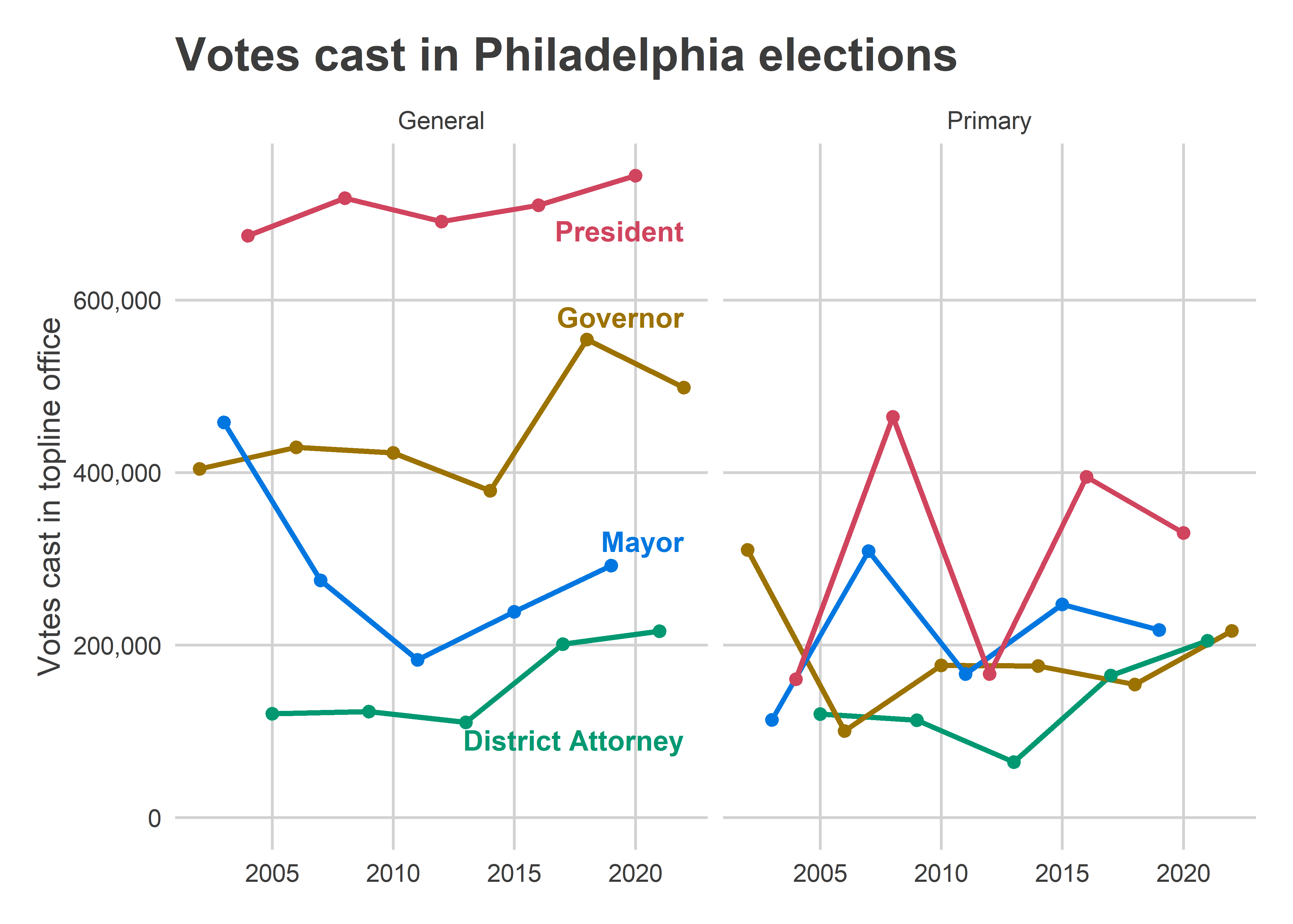
Mayoral primaries usually see the second highest turnout, after Presidential. In the last two competitive mayoral races, 2007 and 2015, we saw 309,000 and 247,000 votes respectively. Given that turnout has dramatically jumped post-2016 and this race is shaping up to be hyper competitive, I’d expect turnout around that 310,000 mark or higher.
How many votes will it take to win?
With so many candidates, the winner won’t need a very high percentage. The two most competitive recent, many-candidate races were 2007 Mayor and 2017 D.A., both with seven candidates. In 2007, Michael Nutter beat Thomas Knox 37% to 25%. In 2017, Larry Krasner beat Joe Khan 38% to 20%. So it looks like it took ~30% to win (halfway between first and second). I’ll call this number the “Win Percent”.
View code
comp_elections <- tribble(
  ~year, ~election_type, ~office,
  "2009", "primary", "DISTRICT ATTORNEY",
  "2017", "primary", "DISTRICT ATTORNEY",
  "2015", "primary", "MAYOR",
  "2007", "primary", "MAYOR",
  "2020", "primary", "PRESIDENT OF THE UNITED STATES",
  "2008", "primary", "PRESIDENT OF THE UNITED STATES",
  "2004", "primary", "PRESIDENT OF THE UNITED STATES",
  "2022", "primary", "UNITED STATES SENATOR",
  "2016", "primary", "UNITED STATES SENATOR",
  "2010", "primary", "UNITED STATES SENATOR",
  "2006", "primary", "UNITED STATES SENATOR",
)

winnum_df <- df_major %>% inner_join(comp_elections) %>%
  filter(
    ifelse(election_type == "primary", party == "DEMOCRATIC"),
    candidate != "Write In"
  ) %>%
  group_by(year, election_type, office, candidate) %>%
  summarise(votes = sum(votes)) %>%
  group_by(year, election_type, office) %>%
  mutate(
    pvote = votes / sum(votes),
    rnk = rank(desc(votes))
  ) %>%
  summarise(
    ncand = length(unique(candidate)),
    winner_pvote = pvote[rnk == 1],
    second_pvote = pvote[rnk == 2]
  ) %>%
  mutate(office_pretty = case_when(
    office == "PRESIDENT OF THE UNITED STATES" ~ "President",
    office == "UNITED STATES SENATOR" ~ "Senate",
    TRUE ~ format_name(office)
  ))

# df_major %>%
#   filter(election_type == "primary", party == "DEMOCRATIC") %>%
#   filter(office == "MAYOR") %>%
#   group_by(year, candidate) %>%
#   summarise(votes = sum(votes))

ggplot(winnum_df,
       aes(x=ncand, y=100*(winner_pvote + second_pvote) / 2)
) +
  geom_point(size=3, color = strong_purple) +
  ggrepel::geom_text_repel(aes(label=paste(year, office_pretty))) +
  theme_sixtysix() +
  expand_limits(y=0, x=c(1,8)) +
  labs(
    title = "With 10+ candidates, the win number could be < 25%",
    subtitle = "Philadelphia Democratic Primaries",
    x = "Number of candidates",
    y = "Win Percent\navg(first place, second place)"
  )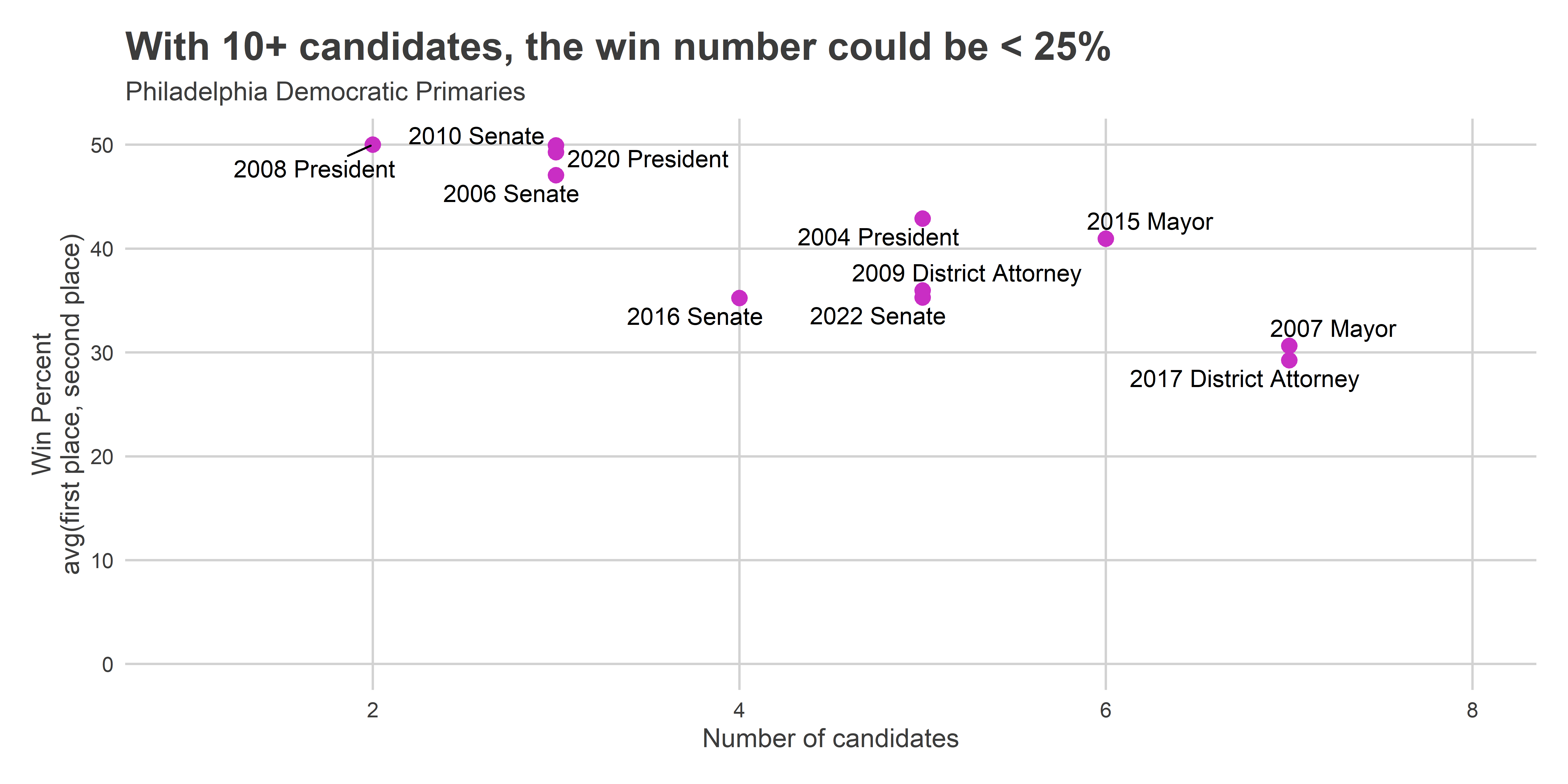
The win percentage at ten candidates looks like it will be 25%, or lower. We haven’t seen 10 candidates in a recent election. If we’re still at or above 10 come May, especially with such high-profile names, that win percent could be as low as 20%.
Where will those votes come from?
Division across the city turn out or stay home in patterns. I’ve analysed these patterns before, creating my voting blocs.
View code
divs <- st_read("../../data/gis/warddivs/202011/Political_Divisions.shp") %>%
  mutate(warddiv = pretty_div(DIVISION_N))source("../../data/prep_data/div_svd_time_util.R")
div_cat_fn <- readRDS("../../data/processed_data/svd_time_20230116.RDS")

div_cats <- div_cat_fn %>% get_row_cats(2017) %>% rename(warddiv = row_id)

cats <- c(
  "Black Voters",
  "Wealthy Progressives",
  "Hispanic Voters",
  "White Moderates"
)

cat_colors <- c(light_blue, light_red, light_orange, light_green)
names(cat_colors) <- cats

ggplot(
  divs %>% left_join(div_cats, by="warddiv")
) +
  geom_sf(aes(fill=cat), color=NA) +
  scale_fill_manual(NULL, values=cat_colors) +
  theme_map_sixtysix() + #%+replace%
  # theme(legend.position="bottom", legend.direction="horizontal") +
  ggtitle("Philadelphia's Voting Blocs")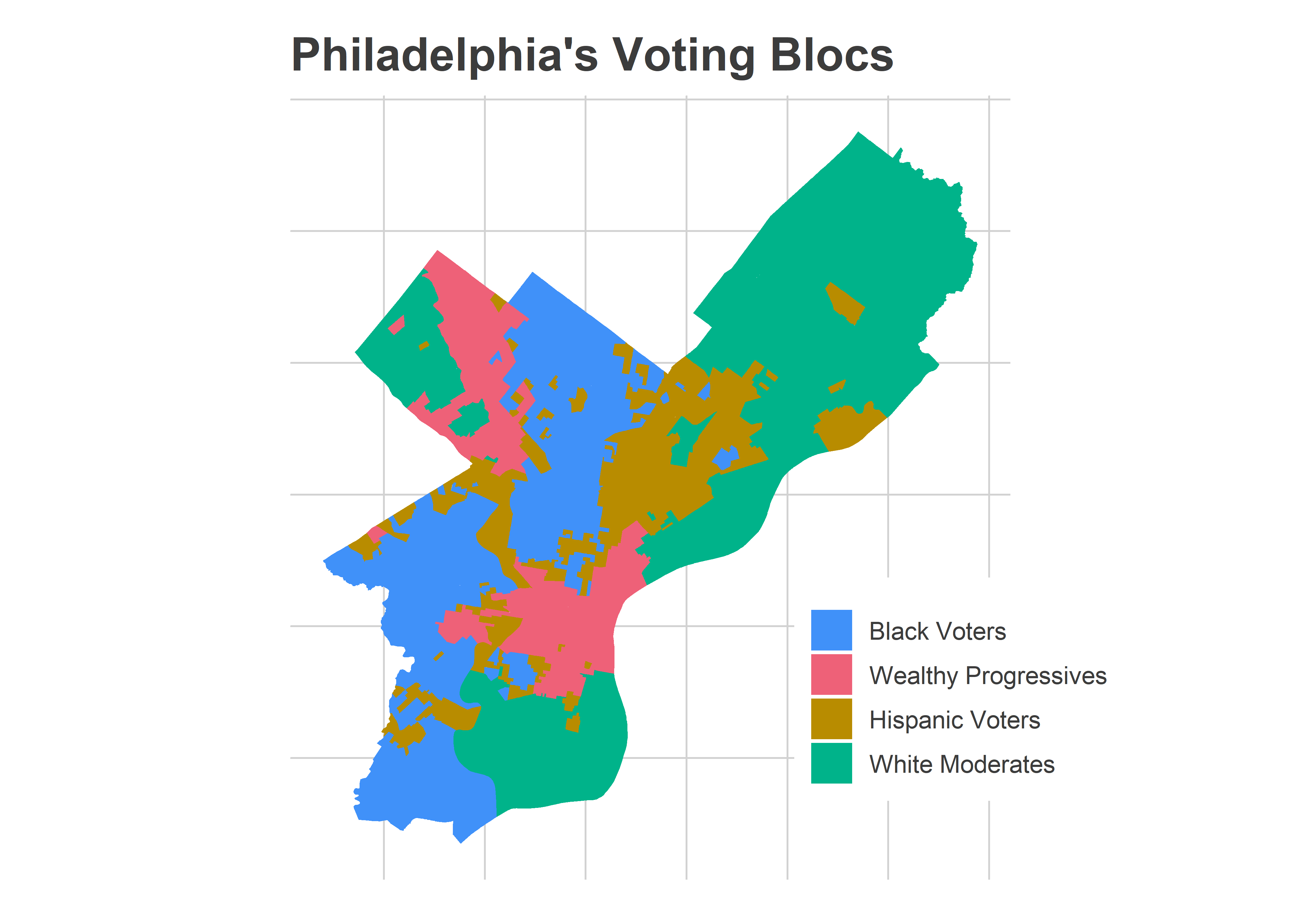
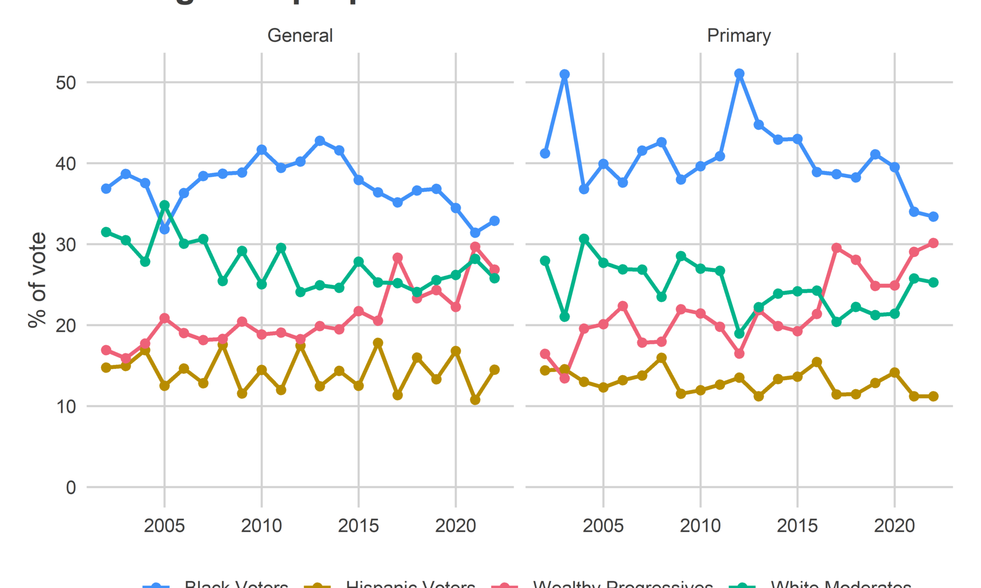
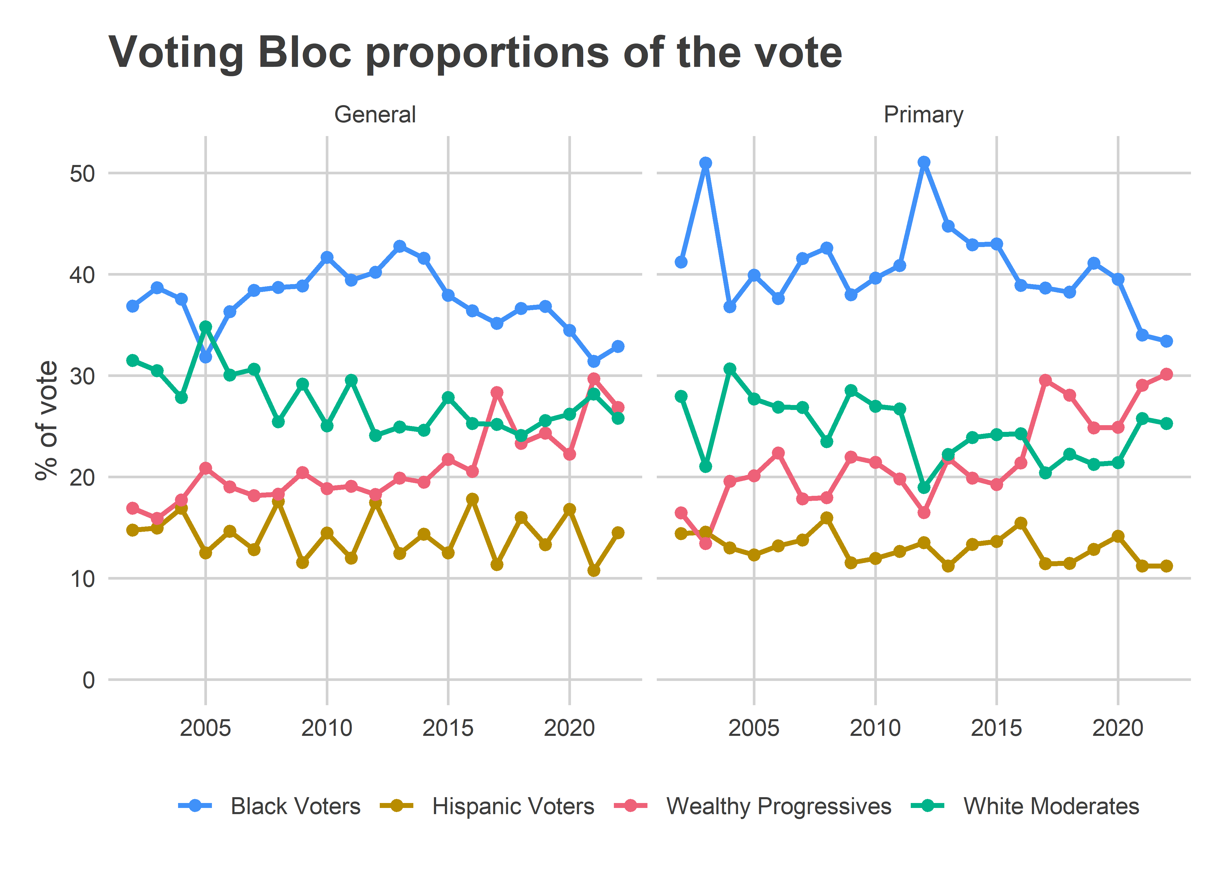
Philadelphia’s Black Wards have had a relatively low proportion of the vote since November 2020. But I expect that to recover a little in a Mayoral primary. Let’s say Black Voter divisions will cast more than 35% of votes, Wealthy Progressives about 30% of the vote, White Moderates 25%, and Hispanic North Philly 10%.
View code
df_major %>%
  filter(is_topline_office) %>%
  left_join(div_cats %>% select(-year), by = "warddiv") %>%
  group_by(year, election_type, cat) %>%
  summarise(votes = sum(votes)) %>%
  group_by(year, election_type) %>%
  mutate(total_votes = sum(votes), pvote = votes / total_votes) %>%
  ungroup() %>%
  filter(!is.na(cat)) %>%
  ggplot(
    aes(x = asnum(year), y = 100*pvote, color=cat)
  ) +
  geom_line(size=1) +
  geom_point(size=2) +
  facet_grid(~format_name(election_type)) +
  theme_sixtysix() +
  scale_color_manual(NULL, values=cat_colors[order(names(cat_colors))]) +
  expand_limits(y=0) +
  labs(
    x = NULL,
    y = "% of vote",
    title = "Voting Bloc proportions of the vote"
  )
The types of possible winners
What kinds of coalitions could put a candidate over the top? Let’s assume a candidate (a) needs 25% of the vote to win, and (b) the breakdown of votes is 35% Black Voter divisions, 30% Wealthy Progressive divisions, 25% White Moderate divisions, and 10% Hispanic Voter divisions.
The winner will be the candidate who achieves \[ 0.35 p_{blk} + 0.30 p_{wprog} + 0.25 p_{wmod} + 0.10 p_{hisp} \ge 0.25, \] where \(p_i\) is the proportion of the vote received in bloc \(i\).
Consider, for example, just the Black Voter and Wealthy Progressive Blocs.
View code
cat_corr_df <- df_major %>%
  inner_join(winnum_df) %>%
  filter(candidate != "Write In", party == "DEMOCRATIC") %>%
  mutate(winnum = (winner_pvote + second_pvote)/2) %>%
  left_join(div_cats %>% select(-year)) %>%
  filter(!is.na(cat)) %>%
  group_by(year, office_pretty, candidate, cat, winnum) %>%
  summarise(votes = sum(votes)) %>%
  group_by(year, office_pretty, cat) %>%
  mutate(total_votes = sum(votes)) %>%
  ungroup() %>%
  mutate(
    pvote = votes / total_votes,
    pvote_norm = pvote / winnum
  ) %>%
  pivot_wider(
    id_cols = c(year, office_pretty, candidate, winnum),
    values_from = c(pvote, pvote_norm, votes),
    names_from = c(cat)
  )

y_prop <- 0.35
x_prop <- 0.30

ggplot(
  cat_corr_df,
  aes(
    x=`pvote_norm_Wealthy Progressives`,
    y=`pvote_norm_Black Voters`
  )
) +
  geom_hline(yintercept = 1.0, color="grey50") +
  geom_vline(xintercept = 1.0, color="grey50") +
  geom_abline(slope = -x_prop / y_prop, intercept = 1 + x_prop/y_prop, linetype="dashed") +
  annotate(
    "text",
    label = "Win Line",
    x=0.05, y=1 +x_prop/y_prop,
    angle= atan(-x_prop / y_prop) * 180 / pi
  ) +
  geom_text(
    aes(label = paste0(format_name(candidate)," ", year)),
    size=3.0
  ) +
  coord_fixed() +
  theme_sixtysix() +
  labs(
    title="Candidate performance in\n Black and Progressive Divisions",
    x = "% of vote in Wealthy Progressive / Win Percent",
    y = "% of vote in Black Voter / Win Percent"
  )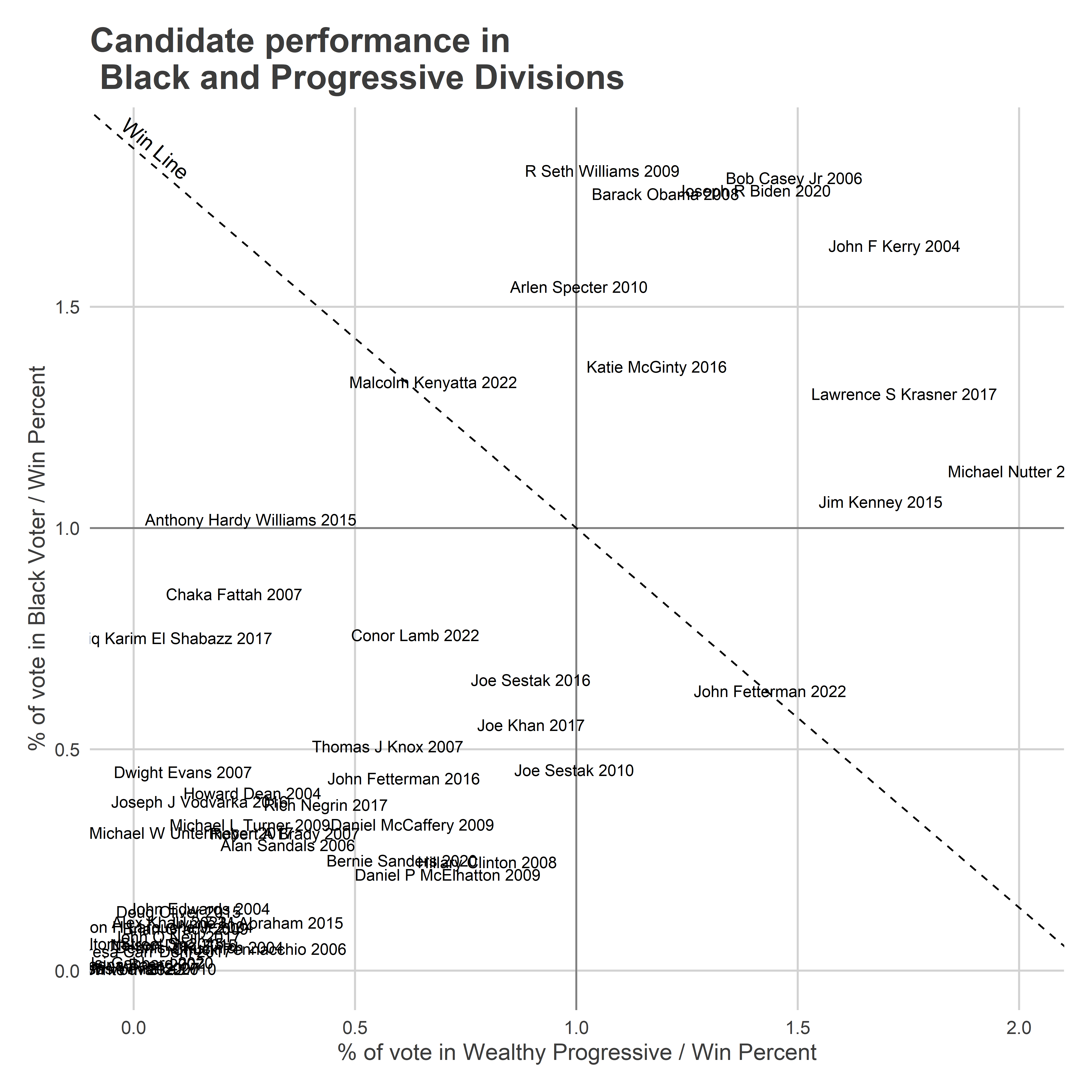
Winning these combined blocs requires being above the dashed line. Williams, Obama, Biden, Kerry, Krasner, Nutter, and Kenney all cleared it easily. Malcolm Kenyatta won these Philadelphia blocs in 2022 by dominating the Black Wards. Fetterman did better in the Wealthy Progressive wards, but not enough to win the head-to-head.
Compare that to the White Moderate and Black Voter comparison. These dimensions are uncorrelated; candidates often do well in one but not the other.
View code
y_prop <- 0.35
x_prop <- 0.25

ggplot(
  cat_corr_df,
  aes(
    x=`pvote_norm_White Moderates`,
    y=`pvote_norm_Black Voters`
  )
) +
  geom_hline(yintercept = 1.0, color="grey50") +
  geom_vline(xintercept = 1.0, color="grey50") +
  geom_abline(slope = -x_prop / y_prop, intercept = 1 + x_prop/y_prop, linetype="dashed") +
  annotate(
    "text",
    label = "Win Line",
    x=0.05, y=1 +x_prop/y_prop,
    angle= atan(-x_prop / y_prop) * 180 / pi
  ) +
  geom_text(
    aes(label = paste0(format_name(candidate)," ", year)),
    size=3.0
  ) +
  coord_fixed() +
  theme_sixtysix() +
  labs(
    title="Candidate performance in\n Black and White Moderate Divisions",
    x = "% of vote in White Moderate / Win Percent",
    y = "% of vote in Black Voter / Win Percent"
  )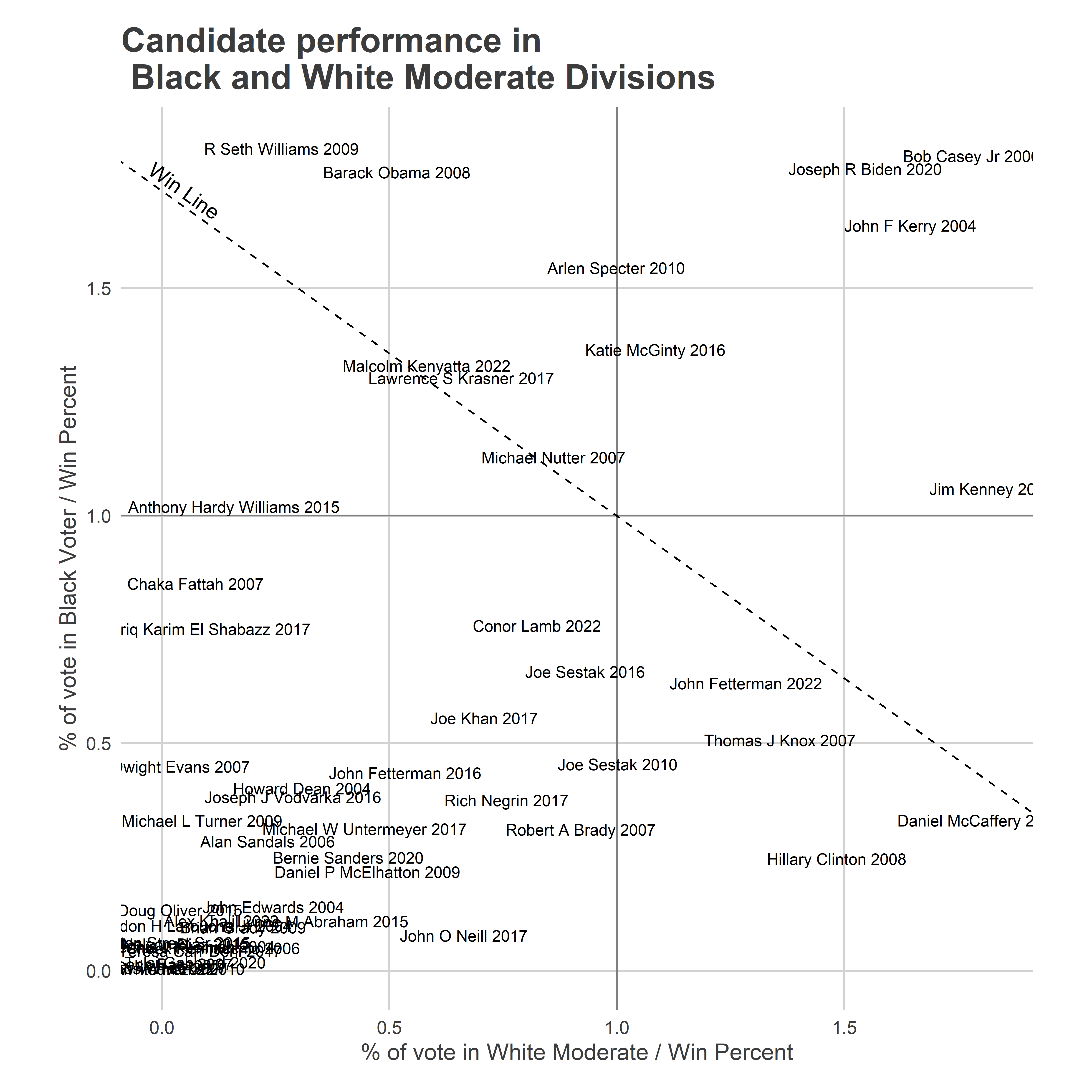
Seth Williams, Barack Obama, Arlen Specter, and even Katie McGinty did well enough in Black Voter divisions to overcome White Moderate weakness. Jim Kenney did much better in White Moderate divisions (although he still beat his win number in Black Voter divisions).
In all cases, an extremely strong showing in a bloc is 1.5 times the win number. This year, that would be 38%. Considering that, here are some combinations of candidates that would win. (To construct these, I’ve taken real candidates’ proportions in each bloc, and adjusted them proportionally up or down to hit exactly win number.)
View code
profiles <- tribble(
  ~candidate, ~year, ~nickname,
  "BARACK OBAMA", "2008", "Black & Progressives",
  "MICHAEL NUTTER", "2007", "Progressive consolidator",
  "ROBERT A BRADY", "2007", "White Moderate consolidator",
  "JOSEPH R BIDEN", "2020", "Party stalwart",
  "ANTHONY HARDY WILLIAMS","2015", "Black consolidator",
  "JOE SESTAK", "2010", "White Moderates & Progressives"
)

profile_res <- cat_corr_df %>%
  inner_join(profiles) %>%
  mutate(candidate=case_when(
    candidate=="ROBERT A BRADY" ~ "BOB BRADY",
    candidate=="JOSEPH R BIDEN" ~ "JOE BIDEN",
    TRUE ~ candidate
  )) %>%
  mutate(total = 0.35 * `pvote_norm_Black Voters` + 0.3 * `pvote_norm_Wealthy Progressives` + 0.25 * `pvote_norm_White Moderates` + 0.1 * `pvote_norm_Hispanic Voters`) %>%
  mutate(
    across(
      `pvote_norm_Black Voters`:`pvote_norm_White Moderates`,
      function(col) col / total * 0.25,
      .names="sim_{.col}"
    )
  ) %>%
  select(candidate, nickname, starts_with("sim_")) %>%
  pivot_longer(
    starts_with("sim_"),
    names_to = "cat",
    values_to = "pvote"
  ) %>%
  mutate(cat = gsub("sim_pvote_norm_", "", cat))

# win_types <- tribble(
#   ~name, ~`Black Voters`, ~`Wealthy Progressives`, ~`White Moderates`, ~`Hispanic Voters`,
#   "Black w enough Progressive", 0.38, 0.20, 0.20, 0.08,
#   "Progressive w some Black", 0.23, 0.38, 0.15, 0.18,
#   "White Moderate with Progressives", 0.08, 0.27, 0.45, 0.27
# ) %>%
#   mutate(
#     total = 0.35 * `Black Voters` + 0.3 * `Wealthy Progressives` + 0.25 * `White Moderates` + 0.1 * `Hispanic Voters`
#   )
# win_types

ggplot(
  profile_res,
  aes(x=cat, y=100*pvote)
) +
  geom_hline(yintercept = 25, linetype="dashed") +
  geom_bar(aes(fill = cat), stat="identity") +
  scale_fill_manual(values = cat_colors, guide=FALSE) +
  geom_text(aes(label = sprintf("%0.0f", 100*pvote)), color="white", vjust = 1.4) +
  facet_wrap(~paste0(nickname, "\n(the \"", format_name(candidate), "\")")) +
  theme_sixtysix() %+replace%
  theme(axis.text.x = element_text(angle=45, hjust=1.1, vjust=1.1))+
  labs(
    title = "Possible Types of Winners",
    x=NULL,
    y="Percent of Vote to win"
  )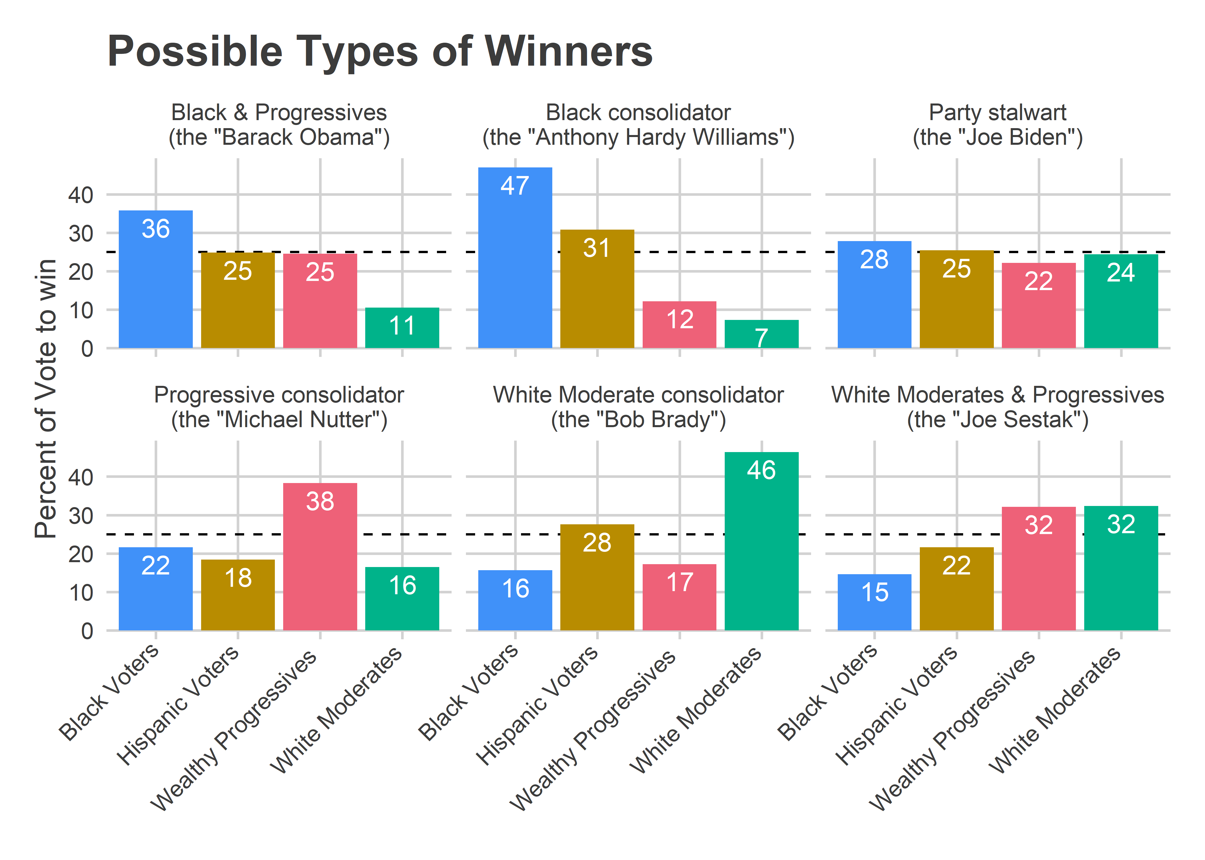
Notice that the single-bloc routes, the
Of course, how easy any of these paths are will depend on how many candidates are vying for them. Are too many candidates vying for the Black-, the Progressive-, or the White Moderate-lane? Coming in Part 2!
I’m hosting a play money market on the Philly mayoral race, and also two on at-large city council races. I’m hoping to engage people and generate some decent forecasts! This is especially useful in elections where there is a lack of polling.
https://manifold.markets/AaronKreider/who-will-win-the-2023-philadelphia
Please join and buy/sell shares based on what you think each candidate’s chances are!