Could a third party win Council At Large?

After an eventful May, Philadelphia’s November General Election will be a lot quieter. The Democrats will almost certainly win every contested race (I’ll look at the interesting District races later), as they do every year.

But the race for the seven Council At Large seats could be more interesting than you think. That’s because the city Charter states that no party can nominate more than five candidates. Historically, this has meant the five Democratic nominees win easily, and two of the five Republicans win. But there’s no reason that the two non-Democrats have to be Republicans, and seven third party or independent candidates have filed petitions to get on the ballot this time around. This includes two candidates from the Working Families Party, which has fielded candidates for the first time.

Before 2015, these candidates wouldn’t have had a shot. But 2015 saw the first non-trivial challenge of the millenium by a third party candidate, with Philadelphia Party candidate Andrew Stober receiving about half the votes of the winning Republican. And the progressives are likely hoping to seize on the success of Larry Krasner who won as a Democrat, but from the progressive wing.

How would it happen? The only plausible way is for Democrats to spend their votes on third party candidates. This would probably be the right strategy for many Philadelphian’s preference sets, using the framework I laid out around Bullet Voting: the Democrats will 100% win, so voting for them has no impact on the state of the world. It’s optimal, then, to spend your votes on candidates with non-zero, non-100% chances. So a progressive might cast votes for all the third party candidates they prefer to Republicans, or the Republican they prefer over others. (Yeah, I know, this logic all changes if every Philadelphian starts thinking this way, and Democrats are then in trouble. I don’t have that kind of readership. The Democrats will win, trust me.)

So, could it really happen? Could enough Democrats strategically cast votes for third party candidates? What would it take? Here’s some data from the recent past.

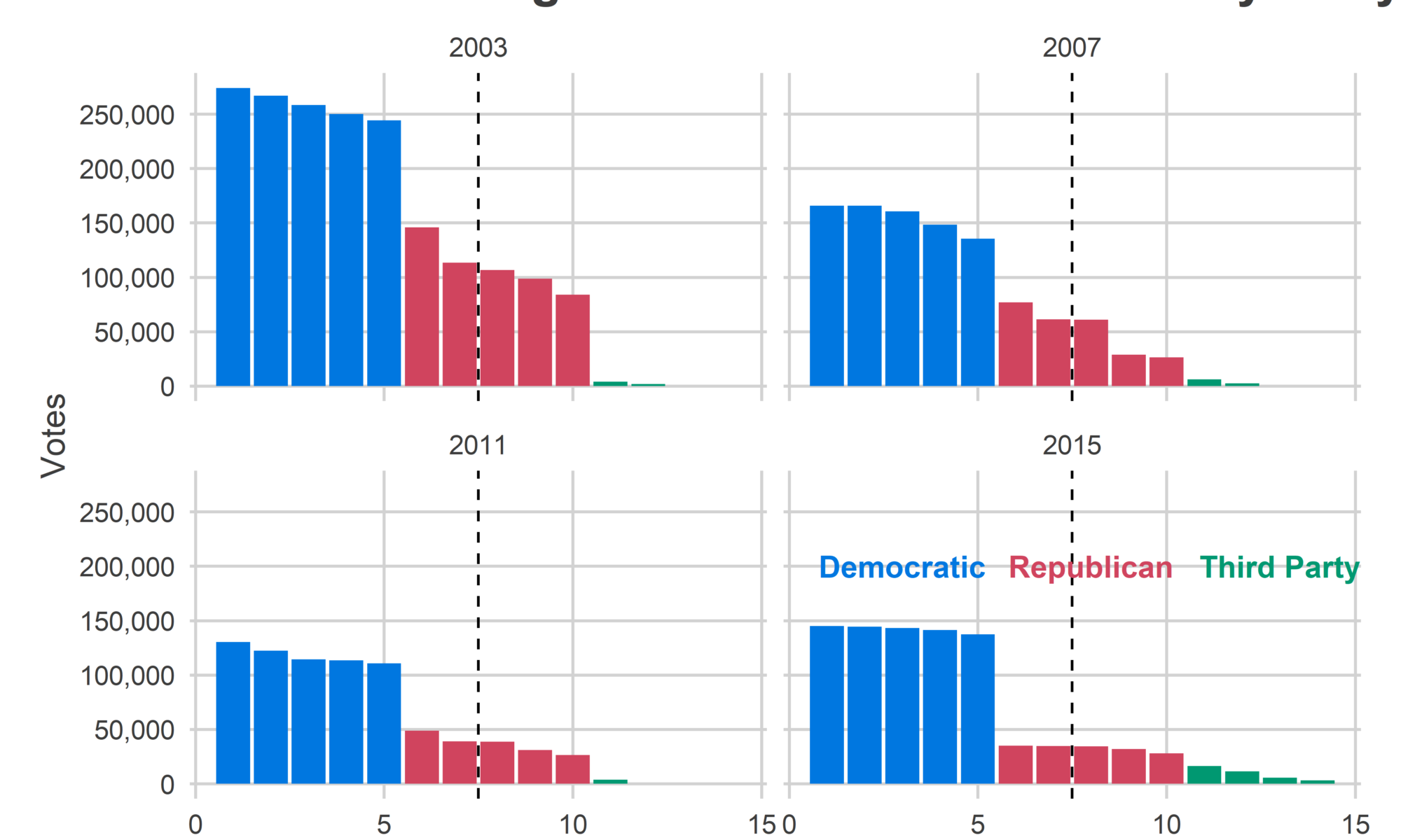
Third Parties didn’t show, until 2015

View code
library(tidyverse)
library(knitr)
library(kableExtra)

df <- safe_load("../../data/processed_data/df_all_2019_07_09.Rda") 

df <- df %>%
  mutate(
    PARTY = ifelse(PARTY == "DEMOCRAT", "DEMOCRATIC", PARTY),
    PARTY = gsub(" PARTY$", "", PARTY)
  )

df_council <- df %>%
  filter(OFFICE %in% c("COUNCIL AT LARGE", "COUNCIL AT-LARGE"), CANDIDATE != "Write In") %>%
  group_by(CANDIDATE, PARTY, WARD19, DIV19, year, election) %>%
  summarise(votes = sum(VOTES)) %>%
  ungroup()

df_total <- df_council %>%
  group_by(CANDIDATE, PARTY, year, election) %>%
  summarise(votes = sum(votes)) %>%
  ungroup()

df_total <- df_total %>%
  mutate(
    CANDIDATE = format_name(CANDIDATE)
  ) %>%
  group_by(year, election) %>%
  mutate(
    rank = rank(desc(votes)),
    pvote = votes/sum(votes)
  ) %>%
  ungroup()

df_total$party_label <- format_name(df_total$PARTY)
df_total$party_label[!df_total$party_label %in% c("Democratic", "Republican")] <- "Third Party" 

colors <- list(
  Democratic=strong_blue, 
  Republican=strong_red,
  `Third Party`=strong_green
)

ggplot(
  df_total %>% filter(election=="general"),
  aes(x=rank, y=votes)
) +
  geom_bar(aes(fill=party_label), stat='identity') +
  facet_wrap(~year) +
  geom_vline(xintercept=7.5, linetype="dashed") +
  theme_sixtysix() +
  xlab("Rank") + ylab("Percent of Vote")+
  scale_y_continuous("Votes", labels=scales::comma, breaks=seq(0,300e3,50e3)) +
  scale_fill_manual(
    "", values=unlist(colors), guide=FALSE
  ) +
  scale_color_manual(
    "", values=unlist(colors),  guide=FALSE
  ) +
  geom_text(
    data=data.frame(
      rank=c(3,8,13), votes=200e3, 
      party_label=c("Democratic", "Republican", "Third Party"),
      year="2015"
    ), 
    aes(label=party_label, color=party_label),
    fontface="bold"
  ) +
  ggtitle("Council At Large General Election Results by Party")
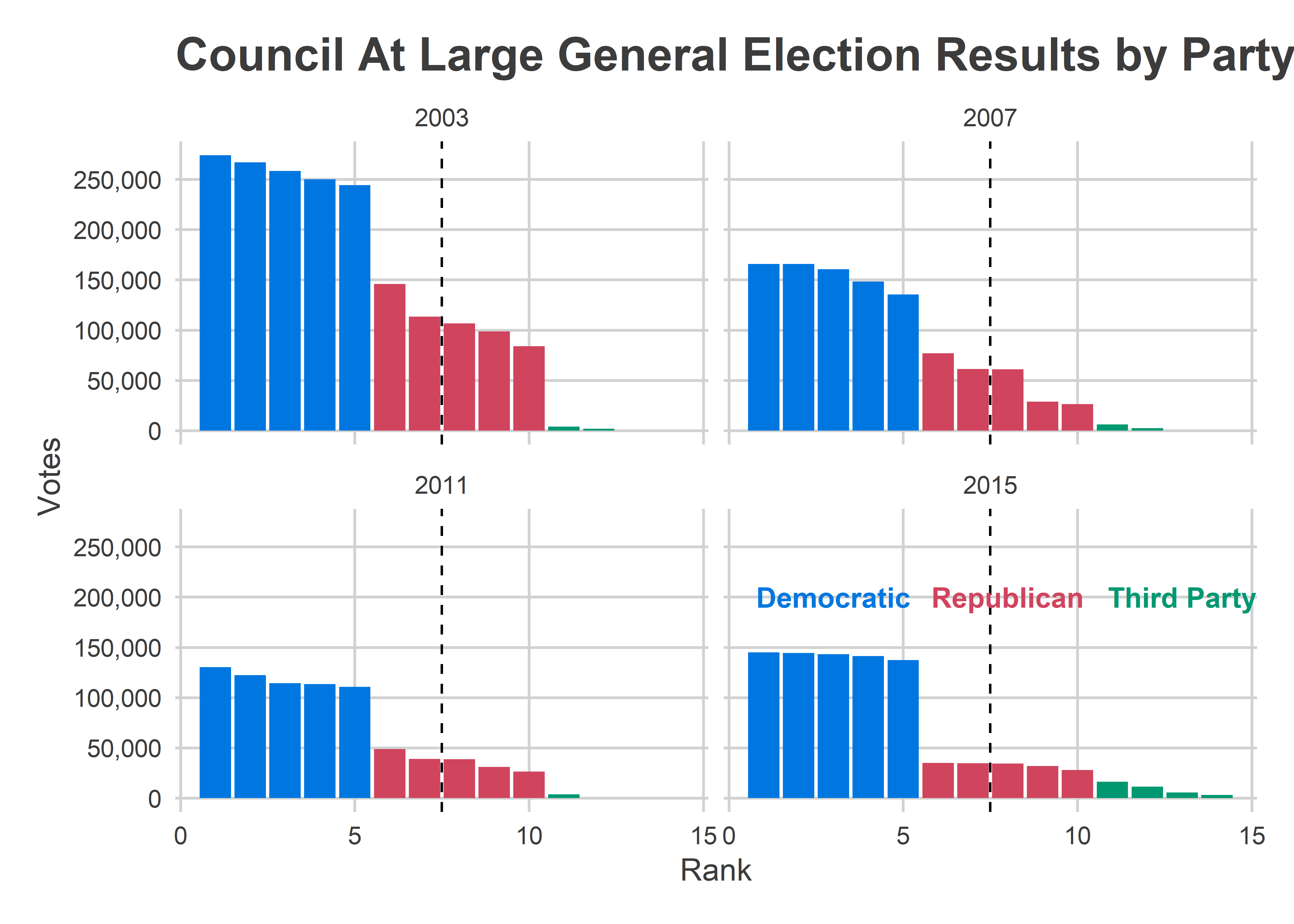
The 2015 election was the first time third party candidates made a stand. Up through 2011, their vote totals don’t break 0.6%, but the 1.8% and 1.2% received by Andrew Stober (Philadelphia Party) and Kristin Combs (Green Party) in 2015 was about 1/2 and 1/3 of the votes needed to win, respectively.

View code
library(knitr)
library(kableExtra)

rank_table <- df_total %>%
  filter(election=="general") %>%
  select(-party_label, -election) %>%
  mutate(
    PARTY = format_name(PARTY),
    pvote=sprintf("%0.1f%%", 100*pvote),
    votes=scales::comma(votes)
  ) %>%
  rename(
    Candidate = CANDIDATE,
    Party = PARTY,
    'Pct Vote' = pvote,
    Votes = votes
  ) %>%
  gather("key", "value", -year, -rank) %>%
  unite("key", year, key, sep = " ") %>%
  spread(key,value, fill = "--")
  
rank_kable <- kable(
  rank_table,
    caption="Recent At Large General Elections",
    align='l',
    col.names=c("Rank", rep(c("Candidate", "Party", "% Vote", "Votes"), times=4)),
    padding = "4in"
  ) %>%
    column_spec(2, width = "1em") %>% 
    add_header_above(
      c(" " = 1, "2003" = 4, "2007" = 4, "2011" =4, "2015" = 4)
    ) %>%
    kable_styling() %>%
    scroll_box(width="100%")

rank_kable
Recent At Large General Elections
2003
2007
2011
2015
Rank Candidate Party % Vote Votes Candidate Party % Vote Votes Candidate Party % Vote Votes Candidate Party % Vote Votes
1 James F Kenney Democratic 14.8% 274,053 Bill Green Democratic 16.0% 165,796 Bill Green Democratic 16.8% 130,403 Helen Gym Democratic 15.9% 145,087
2 David Cohen Democratic 14.4% 266,994 James F Kenney Democratic 16.0% 165,764 James F Kenney Democratic 15.7% 122,384 Derek S Green Democratic 15.8% 144,337
3 W Wilson Goode Jr Democratic 14.0% 258,423 W Wilson Goode Jr Democratic 15.5% 160,531 Blondell Reynolds Brown Democratic 14.7% 114,396 Allan Domb Democratic 15.7% 143,265
4 Juan F Ramos Democratic 13.5% 250,149 Blondell Reynolds Brown Democratic 14.3% 148,236 W Wilson Goode Jr Democratic 14.6% 113,431 Blondell Reynolds Brown Democratic 15.5% 141,368
5 Blondell Reynolds Brown Democratic 13.2% 244,096 William K Greenlee Democratic 13.0% 135,419 William K Greenlee Democratic 14.2% 110,544 William K Greenlee Democratic 15.1% 137,315
6 Frank Rizzo Republican 7.9% 145,852 Frank Rizzo Republican 7.4% 76,937 Dennis M O Brien Republican 6.3% 48,675 David Oh Republican 3.8% 34,887
7 Jack Kelly Republican 6.1% 113,298 Jack Kelly Republican 5.9% 61,239 David H Oh Republican 5.0% 38,835 Al Taubenberger Republican 3.8% 34,711
8 Jamie Mc Dermott Republican 5.8% 106,544 David Oh Republican 5.9% 61,117 Al Taubenberger Republican 5.0% 38,632 Dennis M O Brien Republican 3.8% 34,324
9 David Oh Republican 5.3% 98,687 Patricia A Mattern Republican 2.8% 28,729 Joseph M McColgan Republican 4.0% 30,936 Daniel Tinney Republican 3.5% 31,863
10 David P Hardy Republican 4.5% 83,965 Phil Kerwick Republican 2.5% 26,362 Michael W Untermeyer Republican 3.4% 26,336 Terry Tracy Republican 3.1% 28,050
11 Will Mega Education 0.2% 3,854 Jacinth Brown Roberts Green 0.6% 6,043 Richard Johnson Independent 0.5% 3,627 Andrew C Stober Philadelphia 1.8% 16,301
12 Hilda Cuzco Socialist Workers 0.1% 1,823 Osborne Hart Socialist Workers 0.2% 2,284 Kristin Combs Green 1.2% 11,366
13 Sheila E Armstrong Independent 0.6% 5,466
14 John Staggs Socialist Workers 0.3% 3,028

The raw vote counts needed to win, and even the percentages, bounce around quite a bit. How many votes will it take to win this time? First, how many votes will be cast?

View code
turnout <- df_total %>%
  group_by(year, election) %>%
  summarise(votes = sum(votes))

cycles <- c("President", "DA", "Governor", "Mayor")
get_cycle <- function(year) cycles[(asnum(year) %% 4)+1]

ggplot(
  turnout %>% 
    filter(
      asnum(year) %% 4 == 3
    ),
  aes(x=year, y=votes, color=election)
) +
  geom_point(size=2) +
  geom_line(aes(group=election)) +
  expand_limits(y=0) +
  theme_sixtysix() +
  scale_y_continuous("", labels = scales::comma) +
  xlab("")+
  scale_color_manual(
    "", 
    values=c(general=strong_green, primary=strong_purple),
    guide=FALSE
  ) +
  annotate(
    "text", 
    x = '2015', 
    y=c(500e3, 1100e3), 
    label=c("Primary", "General"), 
    color=c(strong_purple, strong_green),
    fontface="bold"
  ) +
  ggtitle("Votes cast for Council At Large")
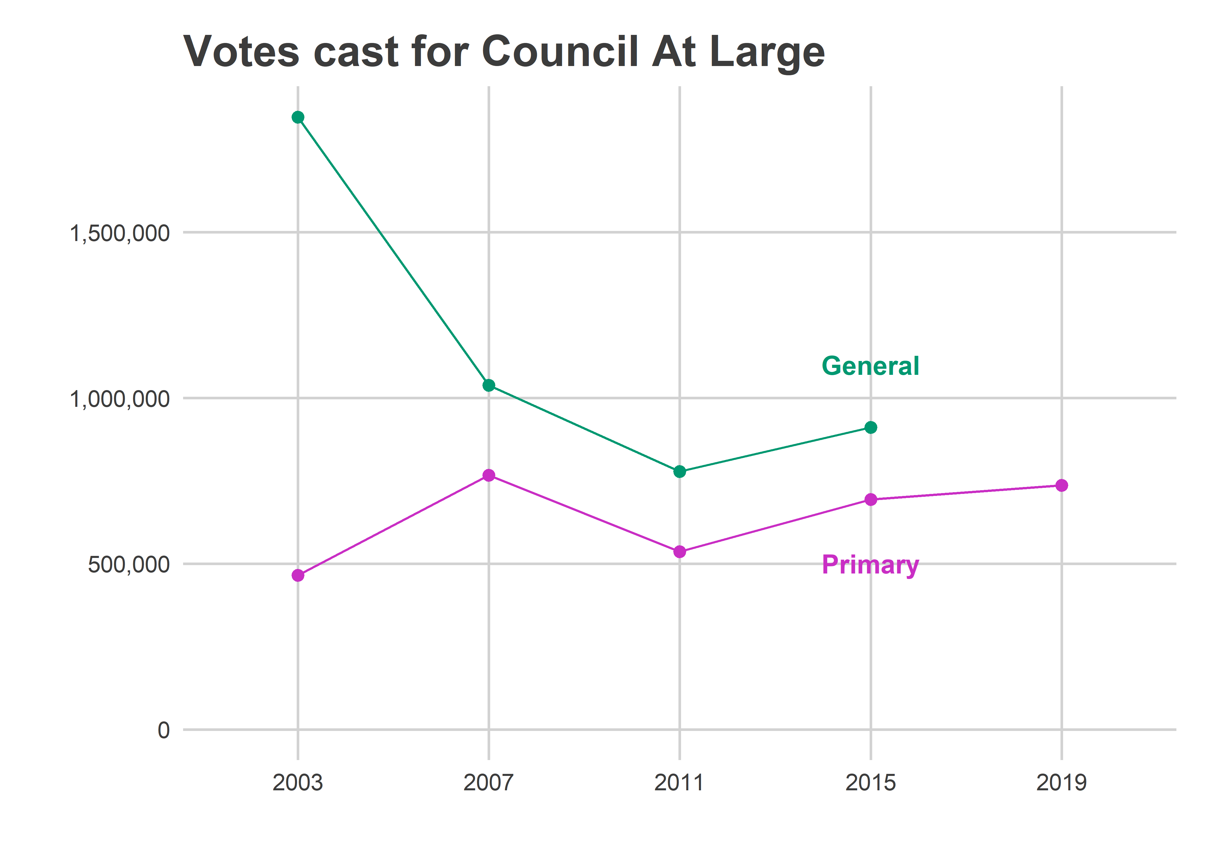
How many votes will be cast in November? The General Election has had about 250,000 more votes cast than the Primary in each of the last three elections. (Notice that votes cast for Council At Large is much higher than the number of voters, since voters can vote for multiple candidates). 2003 had a uniquely competitive General (with Sam Katz challenging John Street), explaining the unique gap that year; that won’t happen this time. We blew past my projections for turnout this past May, with unprecedented excitement for an incumbent-Mayor primary; my hunch is that only a portion of that surge will survive in November, and we’ll see General votes in the 780-800K range.

The At Large win number

How many votes will it take to win the seventh place seat? The five Democrats are guaranteed to win. So the question becomes, how many votes will the second-place Republican get? History can give us a hint. Here are the votes received by Republicans in recent Primary and General Elections, for the topline office and for Council At Large.
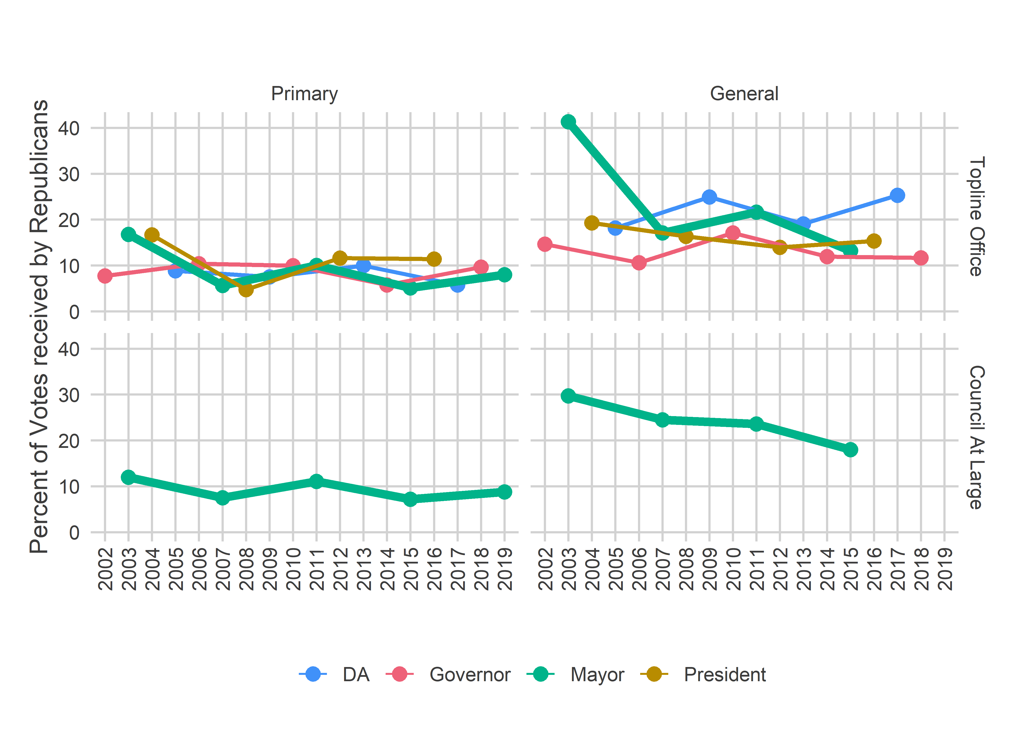
There are two clear trends in the plot above: First, Republicans receive a higher percent of the vote in Mayoral and DA General Elections, presumably because Democratic voters are more variable, and thus turn out in the Presidential and Gubernatorial General Elections, which are always competitive. They turn out less in DA and Mayoral races, where November is rarely competitive.

(Again, ignore 2003, which is an anomaly in every way.)

Second, there has been a steady decline in the percent of the vote received by Republican At Large candidates in the General; there hasn’t been a similar decline in the Primary. This could be two things: 2003 and 2007 Republican votes were helped by Frank Rizzo, who won over 7% of the vote and propped up the Republican average. But also there has been a steady decline in the votes received by the second place Republican in the table above: 6.1%, to 5.9%, to 5.0%, to 3.8%.

What does this mean for the win number? Combining the fact that Republicans win more votes in non-competitive mayoral races with the steady decline, the second place Republican will probably win more than the 3.8% of 2015, but well less than the 5.0% of 2011. With more elections, we could do a statistical estimate, but with only these few, I’ll just make a best guess. My hunch is it’ll be the lower end of the range, let’s say 4.2%. With my turnout guess of 800K, that would be 34K votes.

Where the Third Party votes come from

So the third party candidates need 34K votes. Where would their votes come from?

(Remember, you can find all of these maps and more at the new Sixty-Six Wards Portal!)

Here are Andrew Stober and Kristin Combs’s maps from 2015.

View code
library(sf)
divs <- st_read("../../data/gis/2019/Political_Divisions.shp") %>%
  rename(warddiv = DIVISION_N)df_council <- df_council %>% 
  group_by(year, election, WARD19, DIV19) %>% 
  mutate(pvote = votes/sum(votes))

ggplot(
  divs %>% left_join(
    df_council %>%
      filter(
        year == 2015, 
        election=="general", 
        CANDIDATE %in% c("ANDREW C STOBER", "KRISTIN COMBS")
      ) %>%
      mutate(warddiv = paste0(WARD19, DIV19), Candidate = format_name(CANDIDATE))
  )
) +
  geom_sf(aes(fill = 100 *pvote), color=NA) +
  facet_wrap(~Candidate) +
  scale_fill_viridis_c("Percent\nof Votes") +
  theme_map_sixtysix() %+replace%
  theme(legend.position = "right") +
  ggtitle("Third Party votes come from the Wealthy Progressive Divisions")
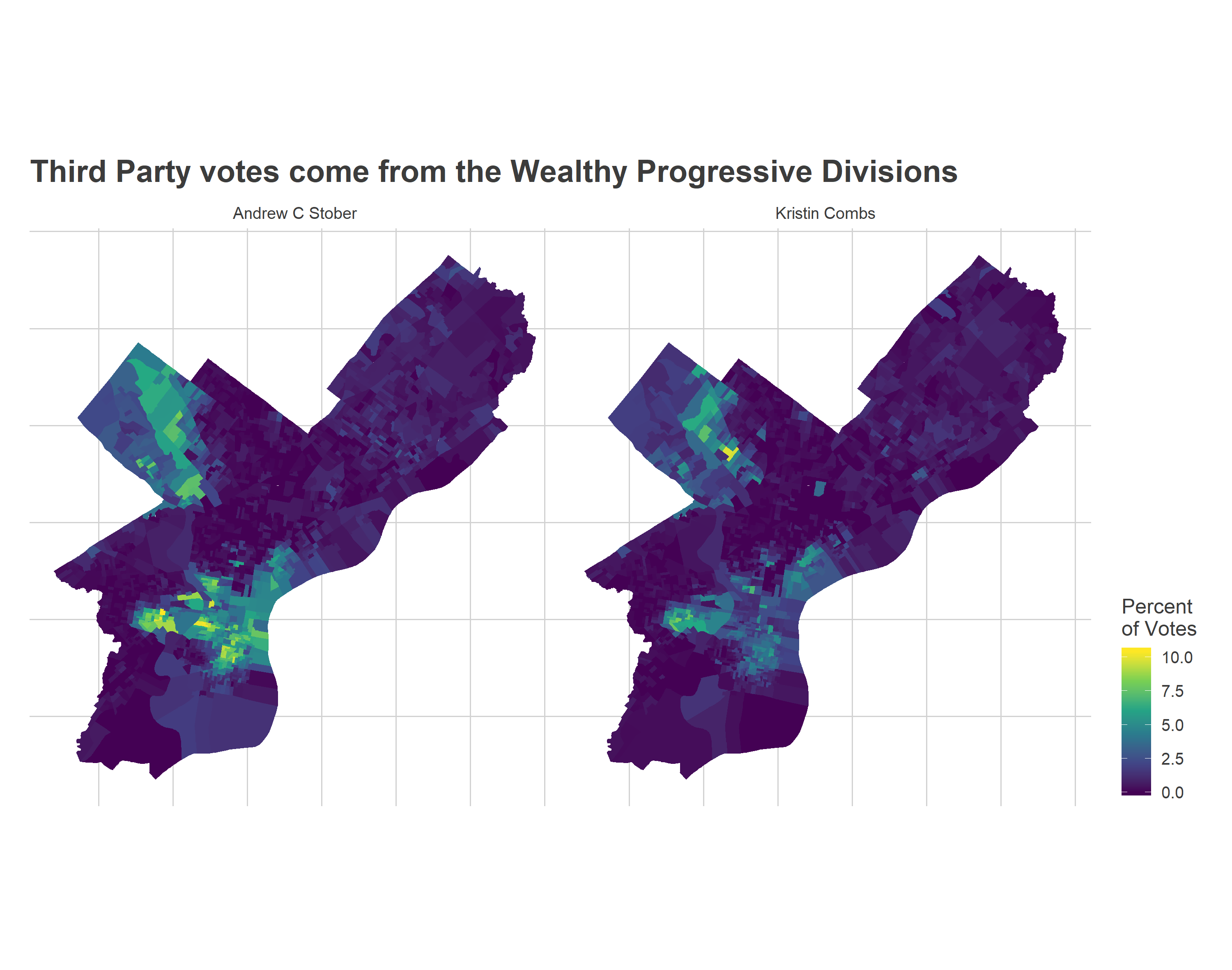
Faithful readers will recognize that basically all of their votes come from the Wealthy Progressive divisions, with an especially heave dependance on University City.

Their maps also look a lot like Krasner’s 2017 map, but with the big exception that they lacking Krasner’s support from some of Philadelphia’s Black Wards, such as the important Northwest Coalition.

View code
ggplot(
 divs %>% left_join(
    df_major %>%
      filter(
        year == 2017, 
        election=="primary", 
        CANDIDATE == c("LAWRENCE S KRASNER")
      ) %>%
      rename(warddiv = warddiv19) %>%
      mutate(Candidate = format_name(CANDIDATE))
  )
) +
  geom_sf(aes(fill = pvote), color=NA) +
  scale_fill_viridis_c("Percent\nof Votes") +
  theme_map_sixtysix() +
  ggtitle("Krasner's results in the 2017 Primary")
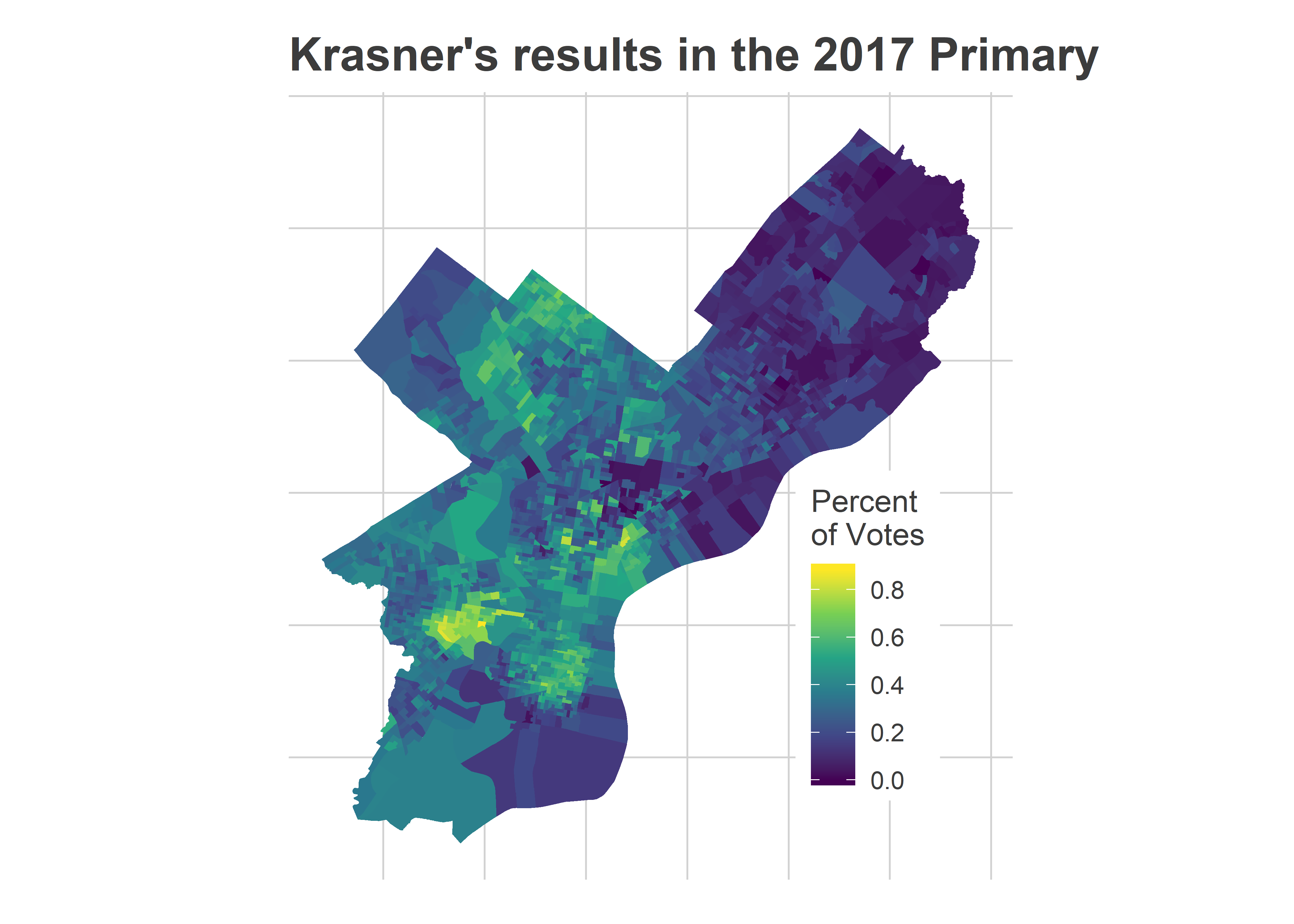
Let’s aggregate the votes to those categories, which shows the heavy differences by voting bloc.

View code
divs_svd <- safe_load("../quick_election_night_maps/divs_svd.Rda")
levels(divs_svd$cat) <- c(
  "Black Voters", "Wealthy Progressives", "White Moderates", "Hispanic North Philly"
)
cat_colors <- c(light_blue, light_red, light_orange, light_green)
names(cat_colors) <- levels(divs_svd$cat)  

divs_svd$warddiv <- divs_svd$DIVISION_N

cat_plot <- bind_rows(
  df_council %>%
    filter(
      year == 2015, 
      election=="general", 
      CANDIDATE %in% c("ANDREW C STOBER", "KRISTIN COMBS")
    ) %>% 
    mutate(warddiv = paste0(WARD19, DIV19)),
  df_major %>%
    filter(year == 2017, election=="primary", CANDIDATE=="LAWRENCE S KRASNER")%>%
    rename(warddiv=warddiv19),
    df_major %>%
    filter(year == 2016, election=="primary", CANDIDATE=="BERNIE SANDERS")%>%
    rename(warddiv=warddiv19)
) %>%
  mutate(
    Candidate = format_name(CANDIDATE),
    div_votes = ifelse(votes==0, 0, votes / pvote)
  ) %>%
  left_join(divs_svd) %>%
  group_by(Candidate, year) %>%
  mutate(citywide_pvote = weighted.mean(pvote, w=div_votes)) %>%
  group_by(Candidate, year, cat) %>% 
  summarise(
    citywide_pvote=citywide_pvote[1],
    cat_votes = sum(votes),
    cat_pvote=weighted.mean(pvote, w=div_votes)
  ) %>%
  ungroup() %>%
  mutate(
    scaled_pvote = cat_pvote / ifelse(Candidate %in% c("Lawrence S Krasner", "Bernie Sanders"), 10, 1),
    Candidate_with_year = sprintf("%s (%s)", Candidate, year)
  )

ggplot(
  cat_plot,
  aes(x=cat, y=100*scaled_pvote)
) +
  geom_bar(stat="identity", aes(fill=cat)) +
  scale_fill_manual("", values=cat_colors) +
  facet_wrap(~Candidate_with_year) +
  theme_sixtysix()%+replace%
  theme(axis.text.x = element_blank()) +
  ylab("Percent of Vote") +
  xlab(NULL) +
  ggtitle("Percent of Vote by Coalition", "Krasner/Sanders's percents scaled down by 10x")
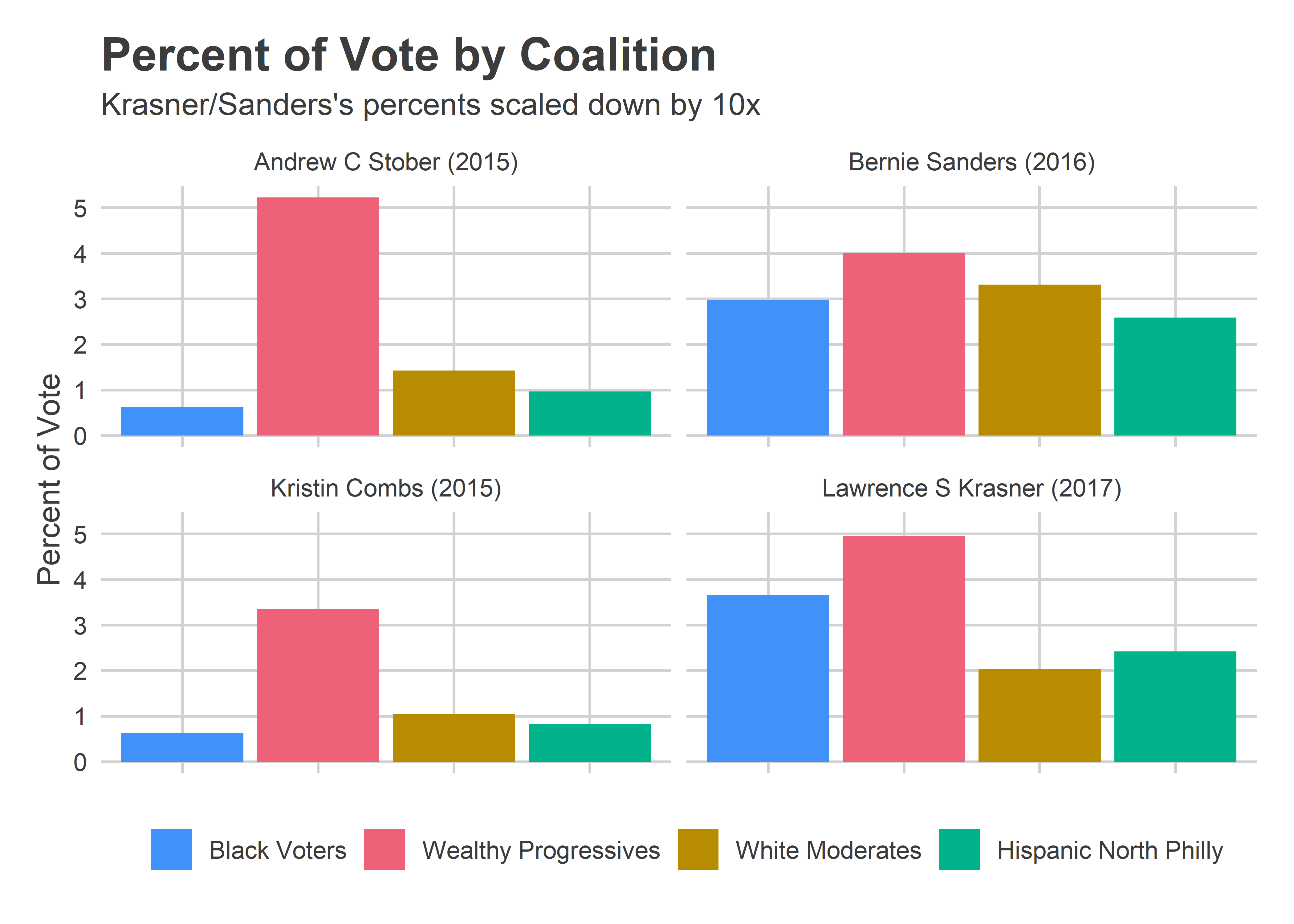
Stober won 5% of the vote from the Wealthy Progressives, but less than 1.5% from each of the other blocs. And his lowest came from the largest bloc, the Black Voters. This is a trend that is likely to continue this year, those Wards are the most consistent voters for the Democratic Party. And with a number of compelling Black candidates on the ballot as Democrats, I’d think it unlikely that too many would additionally cast votes for the third party.

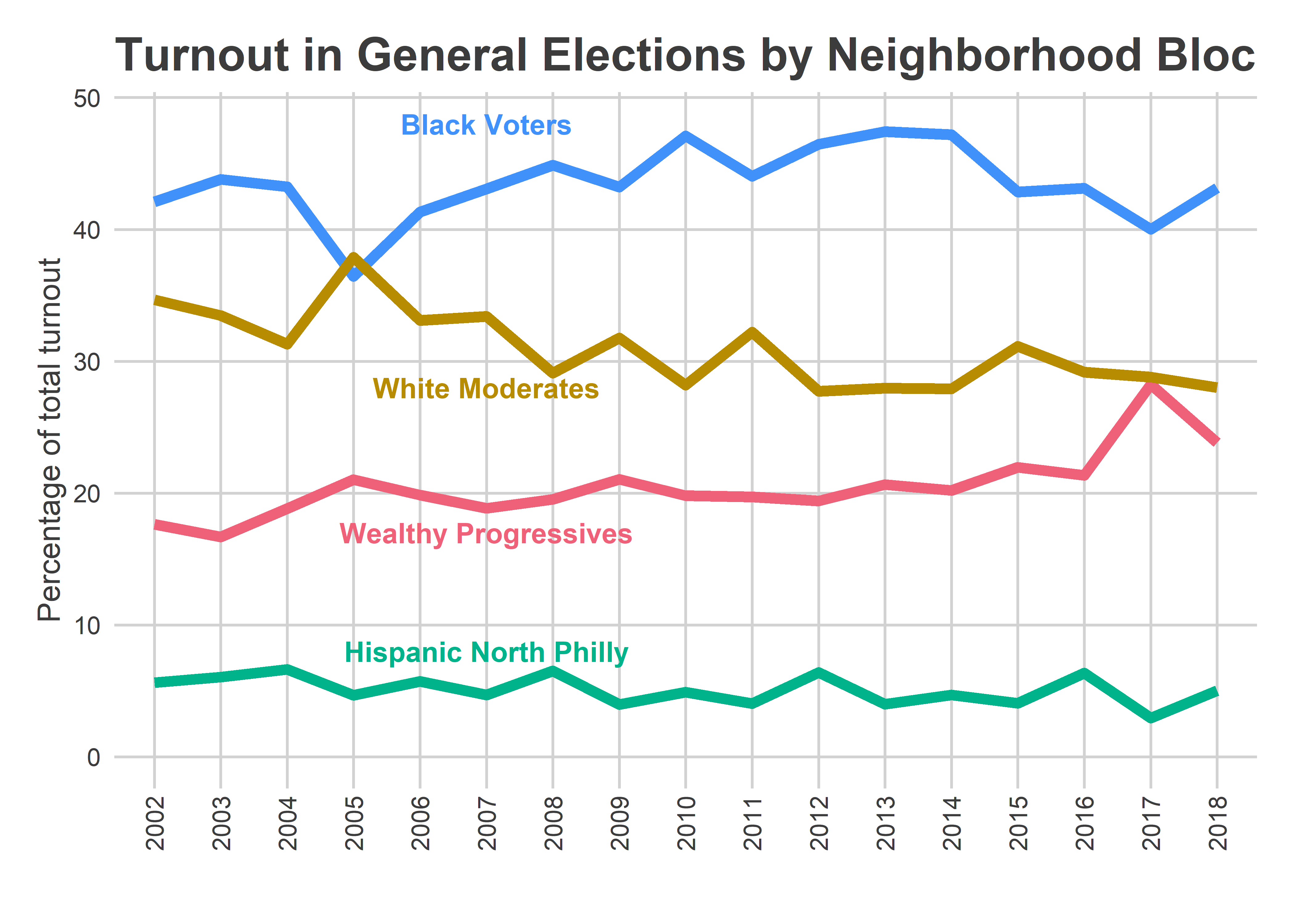
The third party would need those Black Wards to have a shot. The Wealthy Progressive wards that form the third party base have represented only 28 and 24% of the vote in the 2017 and 2018 General Elections, respectively.

View code
turnout_by_cat <- df_major %>% 
  filter(is_primary_office) %>%
  group_by(year, election, warddiv19) %>%
  summarise(votes = sum(votes)) %>%
  left_join(divs_svd, by=c("warddiv19" = "DIVISION_N")) %>%
  group_by(year, election, cat) %>%
  summarise(votes=sum(votes)) %>%
  group_by(year, election) %>%
  mutate(prop=votes/sum(votes)) %>%
  ungroup() %>%
  mutate(
    cycle = get_cycle(year)
  )
  
ggplot(
  turnout_by_cat %>% filter(election == "general"),
  aes(x=year, y=prop*100, color = cat)
) +
  geom_line(aes(group=cat), size=2) +
  annotate(
    geom="text",
    x = "2007",
    y = c(48, 17, 28, 8),
    label = names(cat_colors),
    color=cat_colors,
    fontface="bold"
  ) +
  scale_color_manual("", values=cat_colors, guide=FALSE) +
  scale_y_continuous("Percentage of total turnout") +
  scale_x_discrete("") +
  # facet_wrap(~year) +
  theme_sixtysix() %+replace%
  theme(axis.text.x = element_text(angle = 90)) +
  expand_limits(y=0)+
  ggtitle("Turnout in General Elections by Neighborhood Bloc")
What would it take to win?

Let’s connect all the pieces above.

Let’s assume…

  • Total Turnout: 800K
  • Vote received by 2nd place Republican: 4.2%
  • Third Party receives 0.6% of the vote in Black Voter Divisions, who have 42% of the turnout.
  • Third Party receives 1.2% of the vote in White Moderate Divisions, who have 28% of the turnout.
  • Third Party receives 0.9% of the vote in Hispanic N Philly Divisions, who have 4% of the turnout.

The Black Voter Bloc assumptions may strike you as low, and are crucial to the answer. The Working Families Party’s candidates Kendra Brooks and Nicolas O’Rourke, a Black organizer and Black pastor, respectively, may certainly do better than the White third party candidates of five years ago. On the other hand, these are the Divisions where the Democratic Ward recommendations have the largest effects, and where third parties typically do worst. Plus, they carried Isaiah Thomas and Katherine Gilmore Richardson to victory in May, and may be unlikely to forgo votes for them in November. To be cautious, I’ll consider a second scenario, where the third party candidates double their votes in Black Voter, White Moderate, and Hispanic North Philly Divisions.

Under the assumptions above, the third party candidates win 0.84% of the vote in the non Wealthy Progressive Divisions. To hit 4.0% citywide would require 13% of the vote among the Wealthy Progressive Divisions, or 27,000 of the Divisions’ 208,000 votes cast for At Large. For reference, Krasner received 24,000 votes (50%) from the Wealthy Progressive Divisions in the 2017 Primary.

View code
pvotes = c(0.6, 1.2, 0.9) * 2
turnouts = c(42, 28, 4)

pnonwealthy <- sum(turnouts)/100
pwealthy <- 1 - pnonwealthy

mean_among_nonwealthy <- weighted.mean(pvotes, w=turnouts)
# mean_among_nonwealthy

needed_mean_among_wealthy <- (4.0 - (pnonwealthy * mean_among_nonwealthy)) / pwealthy
# needed_mean_among_wealthy

Hitting that 13% is a huge, likely impossible task. It would require basically every Krasner voter to spend votes on the third party. In 2015, Andrew Stober’s single best Division was 27-01, in which he received 10.4% of the vote (I assume he was standing outside). So to win, this year’s Third Party candidates would have to do better on average across all 280 Wealthy Progressive Divisions than the best 2015 Third Party candidate did in his best Division.

Instead, suppose the third party candidates did twice as well in the Black, White Moderate, and Hispanic divisions. Then they would need 10.6% of the vote from Wealthy Progressives. That is slightly more doable, but still requires them outperforming Stober’s best division, on average.

Could it happen? The only way is with an unprecedented coordination of Democratic voters, sacrificing votes for their party in favor of a strategic vote for their favorite runners up. Nobody came close in 2015 or before, but in a post-2016 world, who knows.
Primary 2019: What was the difference between Common Pleas and Commissioner?

I’ve been stumped by one thing in the months since the Municipal Primary. My high-level story of Council At Large and Commissioner was the dominance of the Party-backed candidates, and the traditional voting strongholds of Philadelphia’s Black and White Moderate neighborhoods. But the story of Common Pleas was the sweep of Bar-endorsees, typically the darling of the Wealthy Progressives, including Tiffany Palmer, a Highly Recommended candidate who won entirely on the back of Center City and the wealthy Northwest.

How can these two exactly opposite stories emerge in the same election? Is one of them wrong? Let’s dig in.

Who won where

First, some maps.

View code
library(tidyverse)
df_all <- safe_load("../../data/processed_data/df_all_2019_07_09.Rda") 

df <- df_all %>%
  mutate(
    OFFICE = ifelse(OFFICE == "COUNCIL AT LARGE", "COUNCIL AT-LARGE", OFFICE)
  ) %>%
  filter(election == "primary" & PARTY == "DEMOCRATIC") %>%
  rename(warddiv=warddiv19, WARD=WARD19, DIV=DIV19) %>%
  group_by(year, OFFICE, CANDIDATE, PARTY, warddiv, WARD, DIV) %>%
  summarise(votes = sum(VOTES))

office_df <- tribble(
  ~office_raw, ~office, ~nwinners,
  "MAYOR", "Mayor", 1,
  "COUNCIL AT-LARGE", "Council At Large", 5,
  "JUDGE OF THE COURT OF COMMON PLEAS", "Common Pleas", 6,
  "CITY COMMISSIONERS", "Commissioner", 2
) %>%
  mutate(office = factor(office, levels=office))

df <- df %>% inner_join(office_df, by = c("OFFICE" = "office_raw"))

##########
## MAPS
##########

# library(leaflet)
# library(leafsync)
library(sf)

divs <- st_read("../../data/gis/2019/Political_Divisions.shp")  %>%
  rename(warddiv=DIVISION_N)wards <- st_read("../../data/gis/2019/Political_Wards.shp") %>%
  mutate(ward = sprintf("%02d", asnum(WARD_NUM)))df <- df %>% 
  group_by(year, warddiv, OFFICE, PARTY) %>%
  mutate(
    div_votes = sum(votes),
    pvote = votes / div_votes
  ) %>% group_by()

df_ward <- df %>% 
  group_by(year, WARD, OFFICE, CANDIDATE, PARTY) %>%
  summarise(votes = sum(votes)) %>% 
  group_by(year, WARD, OFFICE, PARTY) %>%
  mutate(
    div_votes = sum(votes),
    pvote = votes / div_votes
  )


phila_bbox <- st_bbox(divs)

# phila_leaflet <- leaflet() %>% 
#   addProviderTiles(providers$Stamen.TonerLite) %>%
#   setView(
#     lng=mean(phila_bbox[c("xmin", "xmax")]), 
#     lat=mean(phila_bbox[c("ymin", "ymax")]), 
#     zoom = 10
#   )
# 
# add_geom <- function(map, geom, value, pal, text=NA){
#   return(
#     map %>% addPolygons(
#       data = geom, 
#       weight = 0, color = "white", opacity = 1,
#       fillOpacity = 0.8,  smoothFactor = 0.0,
#       popup = text,
#       fillColor = pal(value)
#     )
#   )
# }
# 
# map_candidate <- function(
#   cand_regex,
#   yr, 
#   colname="pvote",
#   pal=NULL,
#   use_divs=FALSE,
#   max_value=1.0
# ){
#   if(use_divs){
#     candidate_df <- divs %>%
#       left_join(
#         df %>% 
#           filter(year == yr, grepl(cand_regex, CANDIDATE)),
#         by=c("warddiv")
#       ) %>%
#       mutate(
#         geo_name = paste0(
#           "Division ", 
#           substr(warddiv, 1, 2), "-", substr(warddiv, 3, 4)
#         )
#       )
#   } else {
#     candidate_df <- wards %>%
#       left_join(
#         df_ward %>% 
#           filter(year == yr, grepl(cand_regex, CANDIDATE)),
#         by=c("ward"="WARD")
#       ) %>%
#       mutate(geo_name = paste("Ward", ward))
#   }
#   
#   candidate_name <- unique(candidate_df$CANDIDATE)
#   
#   if(is.null(pal)) {
#     pal <- colorNumeric("viridis", domain=c(0, max(candidate_df[[colname]])))
#   }
#   
#   text <-  with(
#       candidate_df,
#       paste0(
#         geo_name, "<br>",
#         format_name(CANDIDATE), "<br>", 
#         scales::comma(votes), " vote", ifelse(votes == 1, "", "s"), 
#         " (", round(100*pvote),"%)")
#     )
#   
#   phila_leaflet %>% add_geom(
#     candidate_df$geometry, 
#     pmin(candidate_df[[colname]], max_value), 
#     pal=pal, 
#     text=text
#   ) %>% addControl(format_name(candidate_name), position = "topright")
# }
# 
# map_candidates <- function(cand_regexes, yr, use_divs=FALSE, max_value=NA, ...){
#   all_regex <- paste0("(",cand_regexes,")", collapse = "|")
# 
#   if(is.na(max_value)){
#     if(use_divs) {
#       max_value <- df %>% 
#         filter(year == yr, grepl(all_regex, CANDIDATE)) %>%
#         with(max(pvote))
#     } else {
#       max_value <- df_ward %>% 
#         filter(year == yr, grepl(all_regex, CANDIDATE)) %>%
#         with(max(pvote))
#     }
#   }
# 
#   pal <- colorNumeric("viridis", domain=c(0, max_value))
#   all_maps <- mapply(
#     map_candidate, 
#     cand_regexes, 
#     MoreArgs = list(
#       yr=yr, pal=pal, 
#       use_divs=use_divs, 
#       max_value=max_value
#     ),
#     SIMPLIFY = FALSE
#   )
#   return(all_maps)
# }

map_candidates <- function(cand_regexes, yr, use_divs=FALSE, max_value=NA, ...){
  all_regex <- paste0("(",cand_regexes,")", collapse = "|")

  if(is.na(max_value)){
    if(use_divs) {
      max_value <- df %>%
        filter(year == yr, grepl(all_regex, CANDIDATE)) %>%
        with(max(pvote))
    } else {
      max_value <- df_ward %>%
        filter(year == yr, grepl(all_regex, CANDIDATE)) %>%
        with(max(pvote))
    }
  }

  all_maps <- ggplot(
    wards %>% left_join(
      df_ward %>%
        filter(year==yr, grepl(all_regex, CANDIDATE)),
      by=c("ward"="WARD")
    ) %>%
      mutate(CANDIDATE=format_name(CANDIDATE))
  ) +
     geom_sf(
       aes(fill = 100*pmin(max_value, pvote)),
       color=NA
     ) +
    facet_wrap(~CANDIDATE, ncol = 2) +
    scale_fill_viridis_c(
      "% of Vote"
    ) +
    theme_map_sixtysix() %+replace%
    theme(legend.position = "right")
  return(all_maps)
}

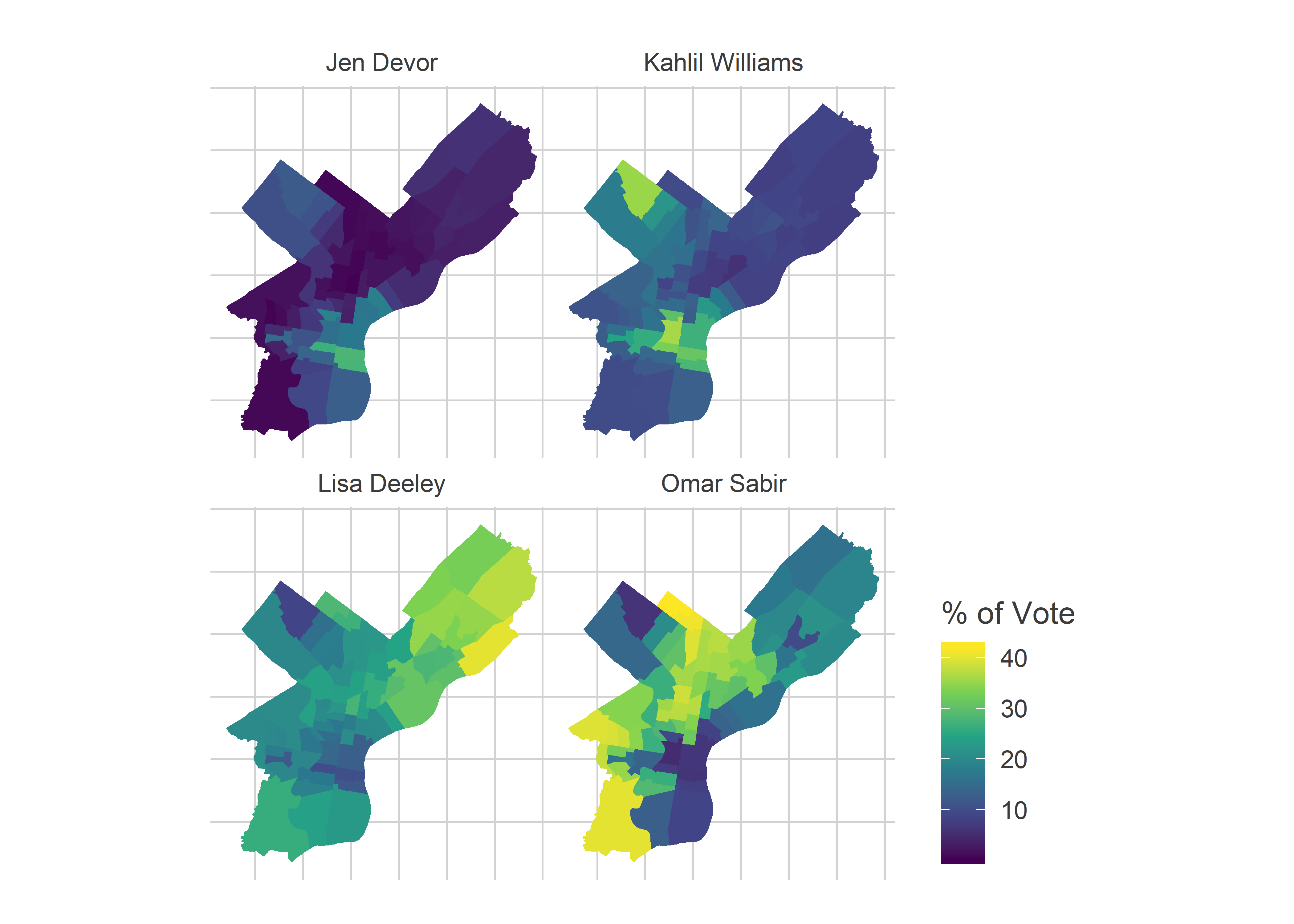
Here are the results for the Commissioner race. Winners Omar Sabir and Lisa Deeley dominated the Black Voter and the White Moderate divisions, respectively. Runners up Khalil Williams and Jen Devor both won the Wealthy Progressive divisions.

[Note: For interactive maps, check out the new Ward Portal! Tables with the results are available in the Appendix.]

2019 Commissioner Results

View code
commissioner_maps <- map_candidates(
  c("SABIR$", "DEELEY$", "KAHLIL.*WILLIAMS$", "DEVOR$"), 
  yr=2019, 
  max_value=0.5
)
commissioner_maps

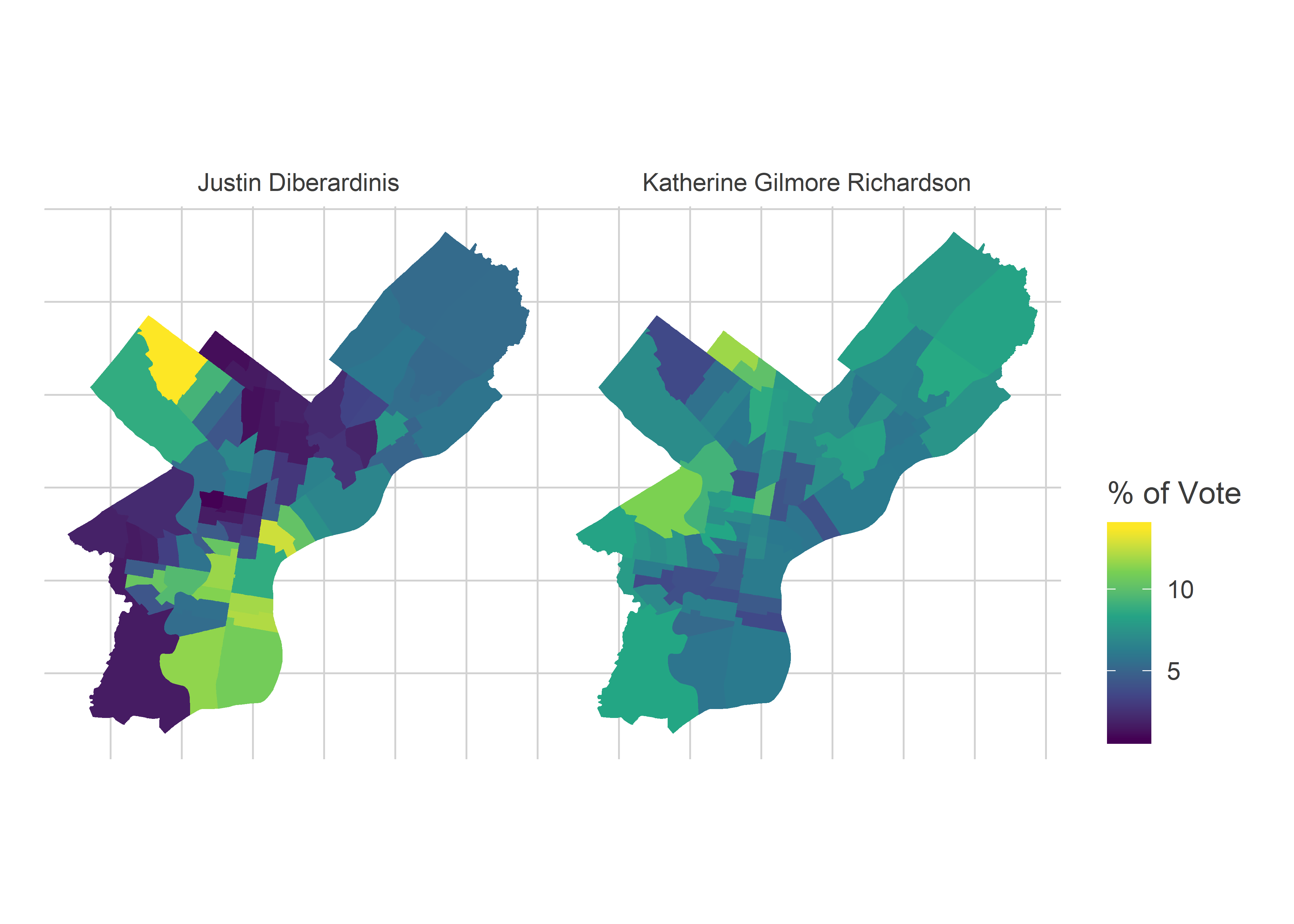
For the Democratic City Council At Large race, the decisive neighborhoods were largely the same. Incumbents Gym, Domb, and Green won across the city, but the two new winners, Thomas and Gilmore Richardson received their highest percents in the Black Voter divisions, while the closest runners up received theirs from the Wealthy Progressives.

(Note: I’ll use the city voting blocs that I’ve discussed before.)

Consider the last in, Gilmore Richardson, versus the first out, Justin DiBerardinis. Gilmore Richardson had more even support across the city than Sabir did, while DiBerardinis attempted to consolidate the Center City and Chestnut Hill/Mount Airy votes, but fell short.

2019 Council Results

View code
council_maps <- map_candidates(
  c("GILMORE RICHARDSON$", "DIBERARDINIS$"), 
  yr=2019, 
  max_value=0.2
)
council_maps

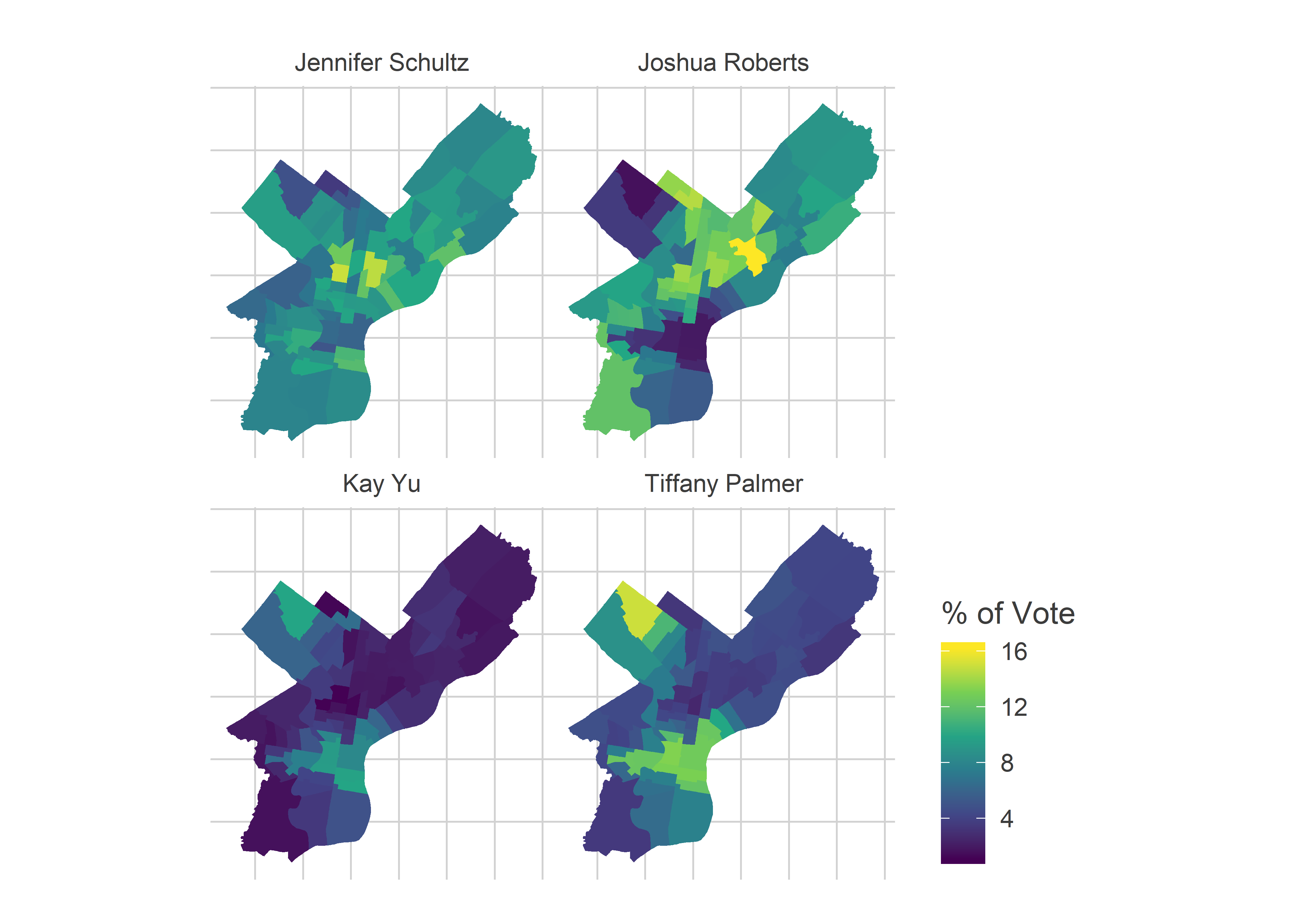
Finally, what did this look like for Common Pleas? Let’s look at four salient candidates: Jennifer Schultz, James Crumlish, Tiffany Palmer, and Kay Yu. The first three won, Yu lost.

2019 Common Pleas Results

View code
commonpleas_maps <- map_candidates(
  c("SCHULTZ$", "ROBERTS$", "PALMER$", "YU$"), 
  yr=2019, 
  max_value=0.2
)
commonpleas_maps

Schultz, with the first ballot position, did well across the city, but especially North Philly. Roberts won places where the DCC nomination matters a lot: the Black Voter and White Moderate divisions. Palmer won a seat with the Wealthy Progressive divisions; Yu’s map looked similar, but she lost.

In some races monopolizing the Wealthy Progressive vote worked, but in other races the votes of the Black Voter divisions dominated. What differentiated them?

Vote power difference by office

My first thought: maybe races have different numbers of votes. Residents could vote for two candidates for Commissioner, five for Council, and six for Common Pleas. In no neighborhoods do voters always vote for the maximum. If voters in different neighborhoods voted for different numbers of candidates, their electoral strength could diverge from just the turnout.

View code
divs_svd <- safe_load("../quick_election_night_maps/divs_svd.Rda") %>%
  mutate(warddiv = paste0(substr(warddiv, 1, 2), substr(warddiv,4,5)))

divs_svd$cat <- forcats::fct_recode(
  divs_svd$cat,
  "Black Voters"="Black non-wealthy",
  "Wealthy Progressives"="Wealthy",
  "White Moderates"="White non-wealthy"
)

cat_colors <- c(light_blue, light_red, light_orange, light_green)
names(cat_colors) <- levels(divs_svd$cat)      

turnout <- safe_load("../voter_db/outputs/turnout_19.rda") %>%
  group_by() %>%
  filter(`Party Code` == "D")

votes_per_office <- df %>% 
  filter(year == 2019) %>%
  filter(!is.na(office)) %>%
  group_by(warddiv, office) %>%
  summarise(votes = sum(votes)) %>%
  group_by() %>%
  left_join(turnout) %>%
  left_join(
    divs_svd %>% as.data.frame() %>% select(warddiv, cat)
  ) %>%
  group_by(cat, office) %>%
  summarise(votes=sum(votes), turnout=sum(turnout)) %>%
  group_by() %>%
  mutate(votes_per_voter = votes / turnout) %>%
  select(cat, votes, turnout, office, votes_per_voter) 

# votes_per_office %>% filter(office == "Mayor") %>%
#   mutate(pturnout = turnout/sum(turnout))
# 
# votes_per_office %>% group_by(office) %>%
#   mutate(pvotes = votes/sum(votes))

ggplot(
  votes_per_office %>% left_join(office_df),
  aes(x=cat, y=votes_per_voter, fill=cat)
) +
  geom_bar(stat="identity") +
  geom_point(aes(y=nwinners), color=NA) +
  geom_text(
    aes(label = sprintf("%0.2f", votes_per_voter)),
    y=0, vjust=-0.4, color="white"
  )+
  facet_wrap(~office, scales = "free_y") +
  scale_fill_manual(NULL, values=cat_colors) +
    theme_sixtysix() %+replace%
  theme(axis.text.x = element_blank()) +
  ylab("Votes / Voter") +
  xlab(NULL) +
  ggtitle("Votes per voter in different neighborhood blocs")

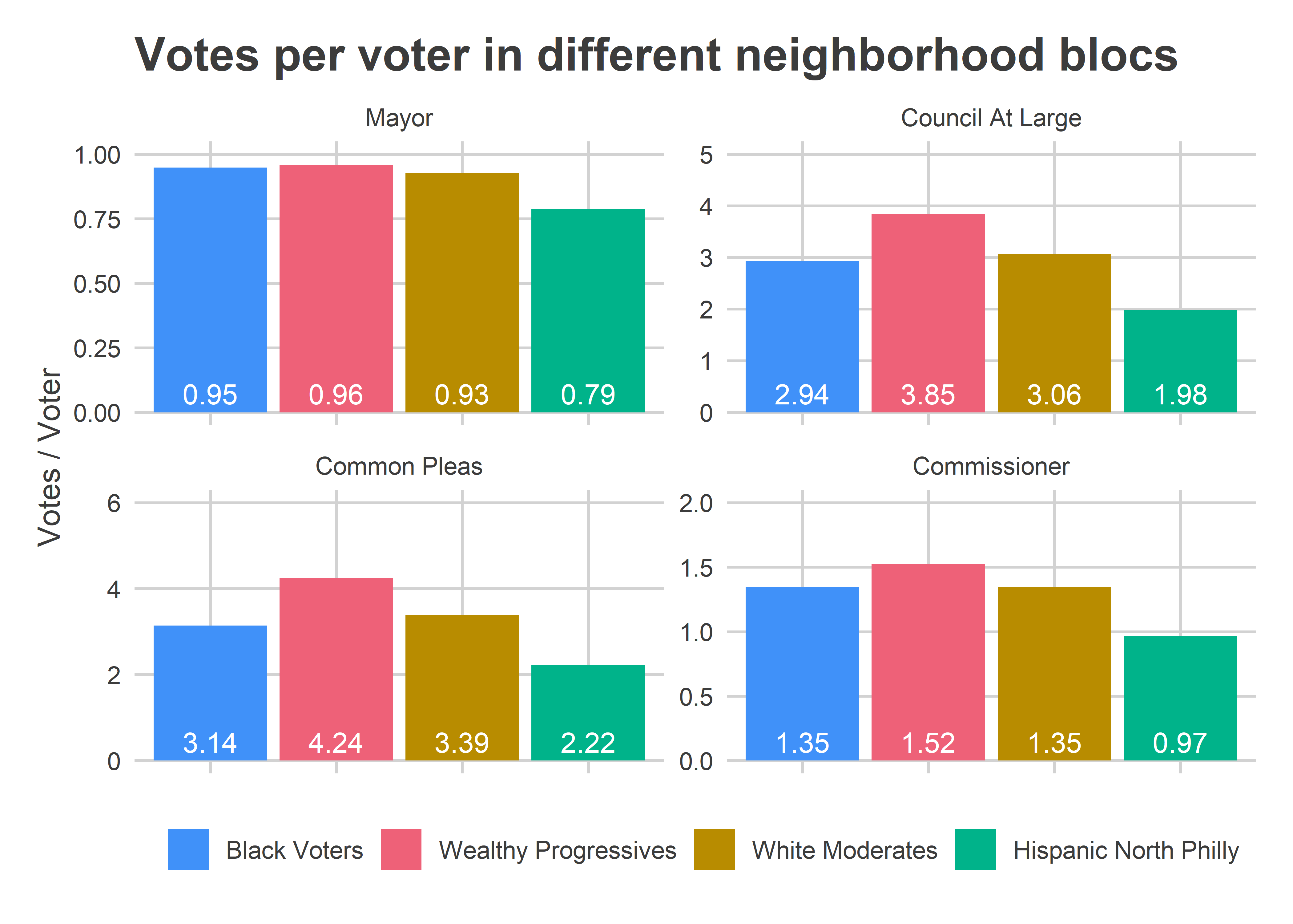
Voting blocs’ numbers are very different by office. The average voter in Black and Wealthy Progressive divisions cast 0.95 and 0.96 votes for Mayor, meaning about 5% of the people who entered the booth left it empty. The rate was basically the same among Black, Wealthy Progressive, and White Moderate divisions.
The rates were not constant for Commissioner. Wealthy Progressive divisions cast 1.52 votes per voter (out of an allowed 2), while Black Voter divisions only cast 1.35.

Wealthy divisions increased that gap even more for Council (voting for 3.9 versus 2.9) and then more for Common Pleas (voting for 4.2 versus 3.1).

Note that I don’t have data for individual voters, so I can’t tell whether this is because some voters skip the race altogether (some vote for 0, others for the full allowance), versus all voters under-voting. We’d need the Commissioner’s Bullet Voting data to adjudicate.

The difference in votes per voter meant that Wealthy Progressive divisions made up 26% of the voters, 26% of the votes for Mayor, 28% of the votes for Commissioner, 31% of the votes for Council at Large, and 32% of the votes for Common Pleas (the Black Voter divisions were 49, 50, 48, 46, and 45, respectively). That’s roughly in order of where their candidates did better: Commissioner worst, Common Pleas best. But the effect isn’t close to strong enough to drive wins except in the narrowest of margins.

One way to visualize that is with scatter plots.

Scatter plots and win lines

I’ve done this before for the Council District Profiles: a twoway scatter mapping the voting blocs of a race. In this case, I’ll plot candidates using their Wealthy Progressive percent on the x-axis, and Black Voter percent on the y-axis. Candidates to the top right do well in both, and win.

View code
cat_df <- df %>% 
  filter(year == 2019) %>%
  mutate(candidate_name = format_name(CANDIDATE)) %>%
  filter(!is.na(office)) %>%
  left_join(
    divs_svd %>% as.data.frame() %>% select(warddiv, cat)
  ) %>%
  group_by(office, candidate_name, cat) %>%
  summarise(votes = sum(votes)) %>%
  group_by(office, cat) %>%
  mutate(
    pvote = votes/sum(votes),
    cat_rank = rank(desc(votes), ties.method = "first")
  )

winner_df <- cat_df %>%
  group_by(office, candidate_name) %>%
  summarise(votes = sum(votes)) %>%
  group_by(office) %>%
  mutate(
    pvote = votes/sum(votes),
    office_rank = rank(desc(votes))
  ) %>%
  left_join(office_df) %>%
  mutate(is_winner = office_rank <= nwinners)

win_lines <- winner_df %>% 
  filter(office_rank %in% c(nwinners, nwinners+1)) %>%
  group_by(office) %>%
  summarise(win_line = mean(pvote))

slopes <- votes_per_office %>%
  select(cat, office, votes) %>%
  spread(key=cat, value=votes) %>%
  mutate(slope=-`Wealthy Progressives`/`Black Voters`) %>%
  left_join(win_lines) %>%
  mutate(
    intercept = win_line * (`Wealthy Progressives`+`Black Voters`) / `Black Voters`
  )

scatter_df <- cat_df %>%
  filter(candidate_name != "Write In") %>%
  select(-votes) %>%
  rename(rank=cat_rank) %>%
  gather("key", "value", pvote, rank) %>%
  unite("key", cat, key) %>%
  spread(key, value) %>%
  mutate(last_name = format_name(gsub("^.*\\b(\\S+)$", "\\1", candidate_name)))

plot_scatter <- function(use_office){
  max_break <- scatter_df %>%
    filter(office==use_office) %>%
    with(max(c(`Wealthy Progressives_pvote`, `Black Voters_pvote`)))
  
  breaks <- seq(0,100,by=ifelse(max_break > 0.2, 10, 5))
  
  ggplot(
    scatter_df %>% filter(office==use_office),
    aes(
      x = 100 * `Wealthy Progressives_pvote`,
      y = 100 * `Black Voters_pvote`
    )
  ) +
    geom_text(
      aes(label = last_name)
    ) +
    geom_abline(
      data=slopes  %>% filter(office==use_office), 
      aes(intercept=100*intercept, slope=slope),
      color="grey50",
      linetype="dashed"
    ) +
    # facet_wrap(~office, scales = "free") +
    coord_fixed() +
    scale_x_continuous(
      "Percent of vote among Wealthy Progressive divisions",
      expand=expand_scale(mult=c(0.05, 0.2)),
      breaks=breaks
    ) +
    scale_y_continuous(
      "Percent of vote among Black Voter divisions",
      breaks=breaks
    ) +
    expand_limits(x=0,y=0) +
    theme_sixtysix() +
    ggtitle(sprintf("Voting Bloc results for %s", use_office))
} 

plot_scatter("Commissioner")

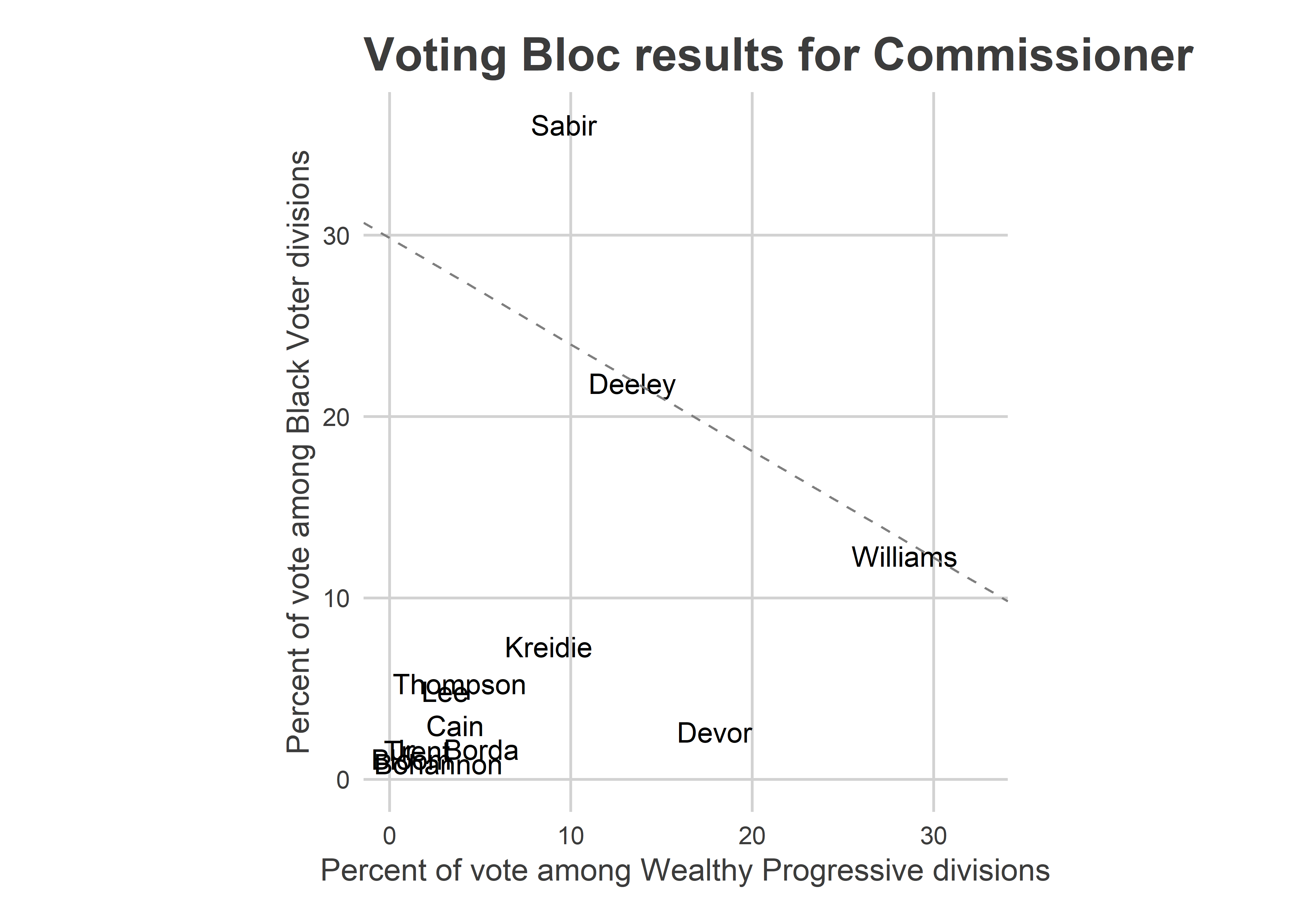
The plot above shows the Commissioner results. The diagonal line is the win line; its slope depends on the relative turnout of the two blocs.

Sabir cleared the line easily, and won. Deeley and Williams ran head-to-head among these blocs (Deeley pulls ahead when you add in the White Moderate divisions).

This race is where the Wealthy Progressive results start to look like vote splitting: Williams and Devor didn’t consolidate the vote of the Wealthy Progressive divisions the way Sabir and Deeley consolidated Black Voter and White Moderate divisions. Had Williams won the 36% among the Wealthy Progressive divisions that Sabir won in Black Voter divisions, that would have been another 6,700 votes. That still wouldn’t have won the race for himc, but would have shrunk the gap behind Deeley by half.

(Note that it’s not clear “vote splitting” happened, since voters could vote for two candidates. So it’s not like the votes for Devor or Kreidie would have otherwise gone to Williams. There probably is at least some substitution effect, though.)

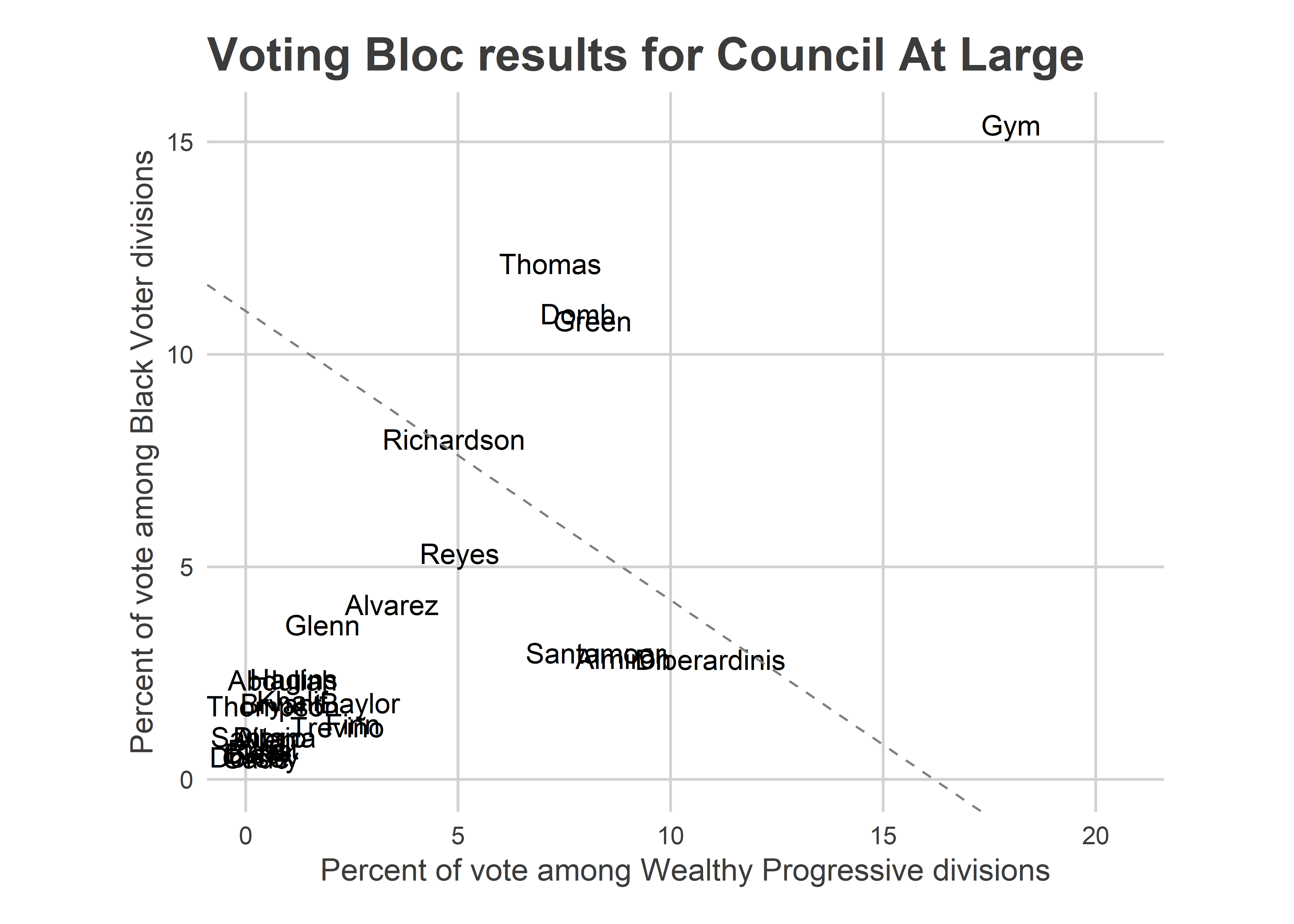
Council has a similar plot, where the runners up clustered just below the line.

View code
plot_scatter("Council At Large")

DiBerardinis, Almiron, and Santamoor are the three candidates clustered around 10% in the Wealthy Progressive divisions. Again, we don’t know that they canibalized votes from each other, since voters could choose five candidates. But since voters only pushed the button for 3.85 candidates on average, there was likely substitution among them happening (plus Gym). Of course, Thomas, Domb, and Green also did relatively well in the Wealthy Progressive divisions, which made their overall wins dominant.
For Common Pleas:

View code
plot_scatter("Common Pleas")

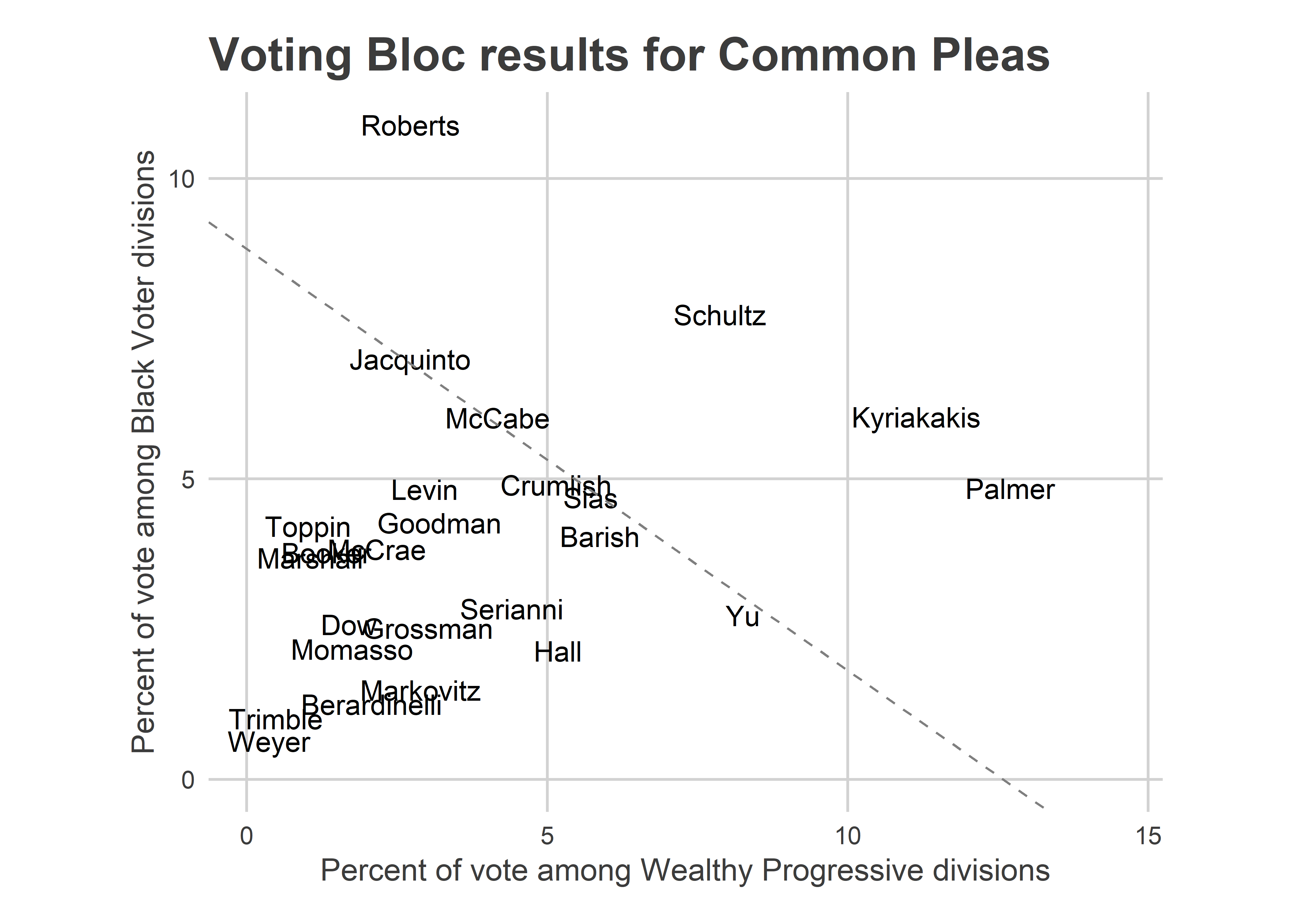
This plot makes it seem that maybe Common Pleas wasn’t different from the other races after all. My original intuition that CP was different was that because the Highly Recommended candidates did so well, and because of Tiffany Palmer’s map, Wealthy Progressives were the determining factor. But this plot shows that they didn’t win solely on the back of Wealthy Progressive neighborhoods. Instead, Palmer finished a strong 7th place among Black Voter divisions, too. The last two judges to win, Crumlish and Jacquinto, were 6th and 3rd in Black Voter divisions, respectively.

Consolidating the vote

One last way to understand vote splitting is a plot of the concentrations of votes in each division. If a voting bloc were able to coordinate their votes so that, for example, their top five Council candidates received 20% of the vote each and everyone else received 0%, that would maximize their power versus the other blocs. If instead they “waste” votes on the sixth and later, then blocs that better consolidate will have more power. Obviously, perfect consolidation won’t happen, but we can look at what percent of the total vote was captured by the winning candidates in each group.

Vote concentration can give a hint at vote splitting. But again, calling it vote splitting assumes that the voters within a bloc have the same preferences, which obviously isn’t true. If one voting bloc has more diversity among voters’ top candidates, that would also hurt this vote consolidation metric.

View code
plot_office <- "Council At Large"

# cat_df %>%
#   filter(office == plot_office) %>%
#   group_by(cat) %>%
#   summarise(
#     pvote_one = sum(pvote * (cat_rank == 1)),
#     pvote_winners = sum(pvote * (cat_rank > 1 & cat_rank <= 5)),
#     pvote_losers = sum(pvote * (cat_rank > 5))
#   )


get_office_plot <- function(
  plot_office, df=cat_df, title="Vote Concentration for %s", show_appendix_text=TRUE
){
  ggplot(
    df %>% filter(office == plot_office),
    aes(x=cat_rank, y=pvote*100, fill=cat)
  ) +
    geom_bar(stat="identity") +
    facet_wrap(~cat) +
    scale_fill_manual(NULL, values=cat_colors, guide=FALSE) +
    geom_vline(
      xintercept=0.5 + office_df$nwinners[office_df$office==plot_office], 
      linetype="dashed"
    ) +
    theme_sixtysix() %+replace%
    theme(axis.text.x = element_blank()) +
    xlab(
      paste0(
        "Candidates sorted by within-cluster rank",
        ifelse(show_appendix_text, "\n(See appendix for names and counts.)", "")
      )
    ) +
    ylab("Percent of Vote") +
    ggtitle(
      sprintf(title, plot_office)
    )
}
get_office_plot("Council At Large")

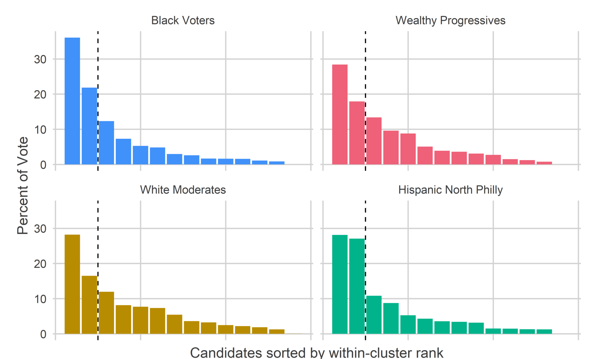
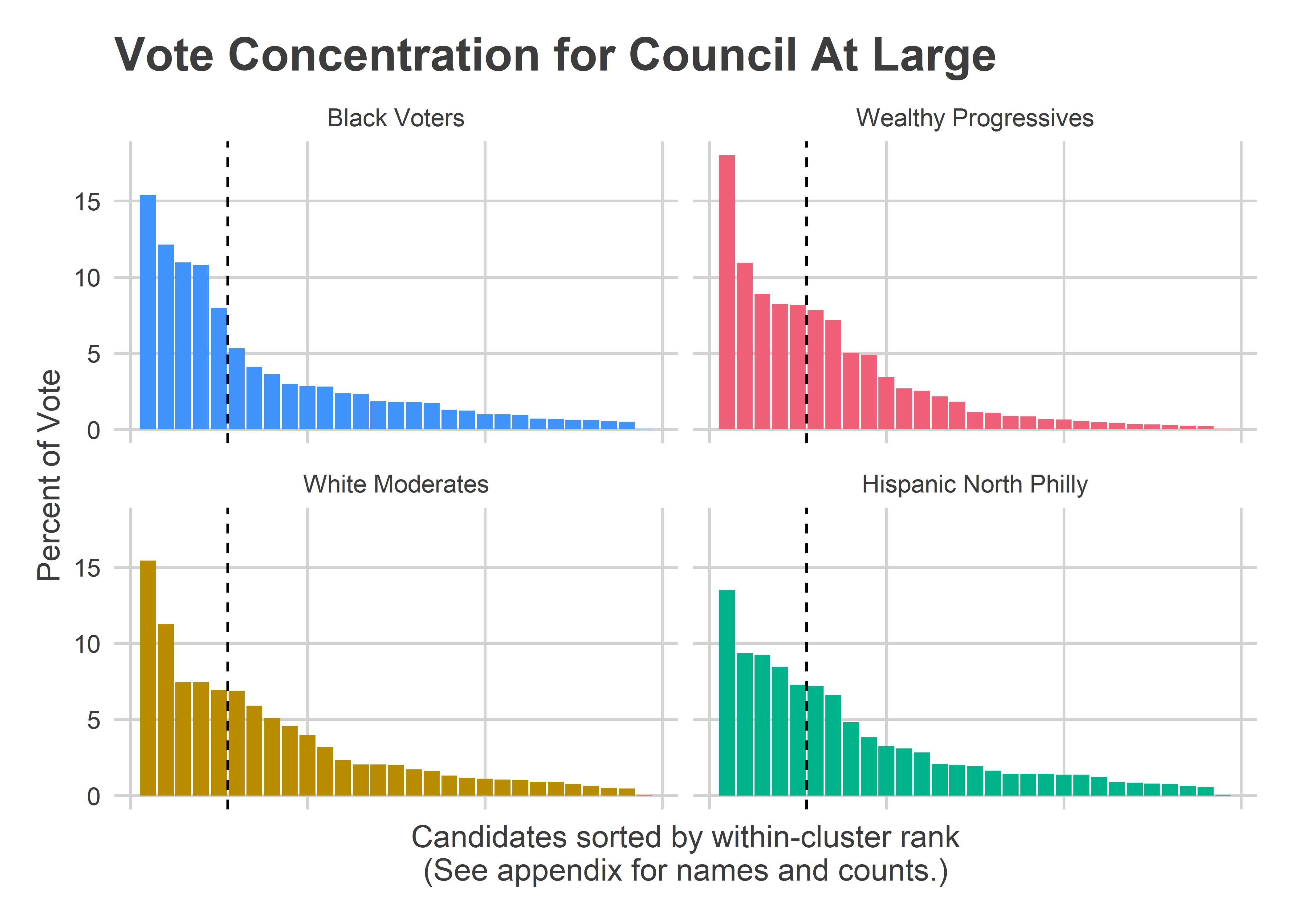
The Black Voter divisions cast 40% of their votes for their 2nd-5th candidates, and 45% of their votes for candidates 6+. The Wealthy Progressive divisions cast 36% of their votes for 2-5, and 46% of their votes for candidates 6+ (Helen Gym was 1st in all of the divisions, and skews the numbers). (For a table with the data behind these plots, see the Appendix.)

Four years ago, those numbers were 40% for the Black Voter 2-5, and 38% for the White Progressive 2-5. So about half the gap, but not enough to swing the election.

Commissioner is the office where there is the best evidence of Wealthy Progressive vote splitting.

View code
# cat_df %>%
#   filter(office == "Commissioner") %>%
#   group_by(cat) %>%
#   summarise(
#     pvote_winners = sum(pvote * (cat_rank <= 2)),
#     pvote_losers = sum(pvote * (cat_rank > 2))
#   )

get_office_plot("Commissioner")

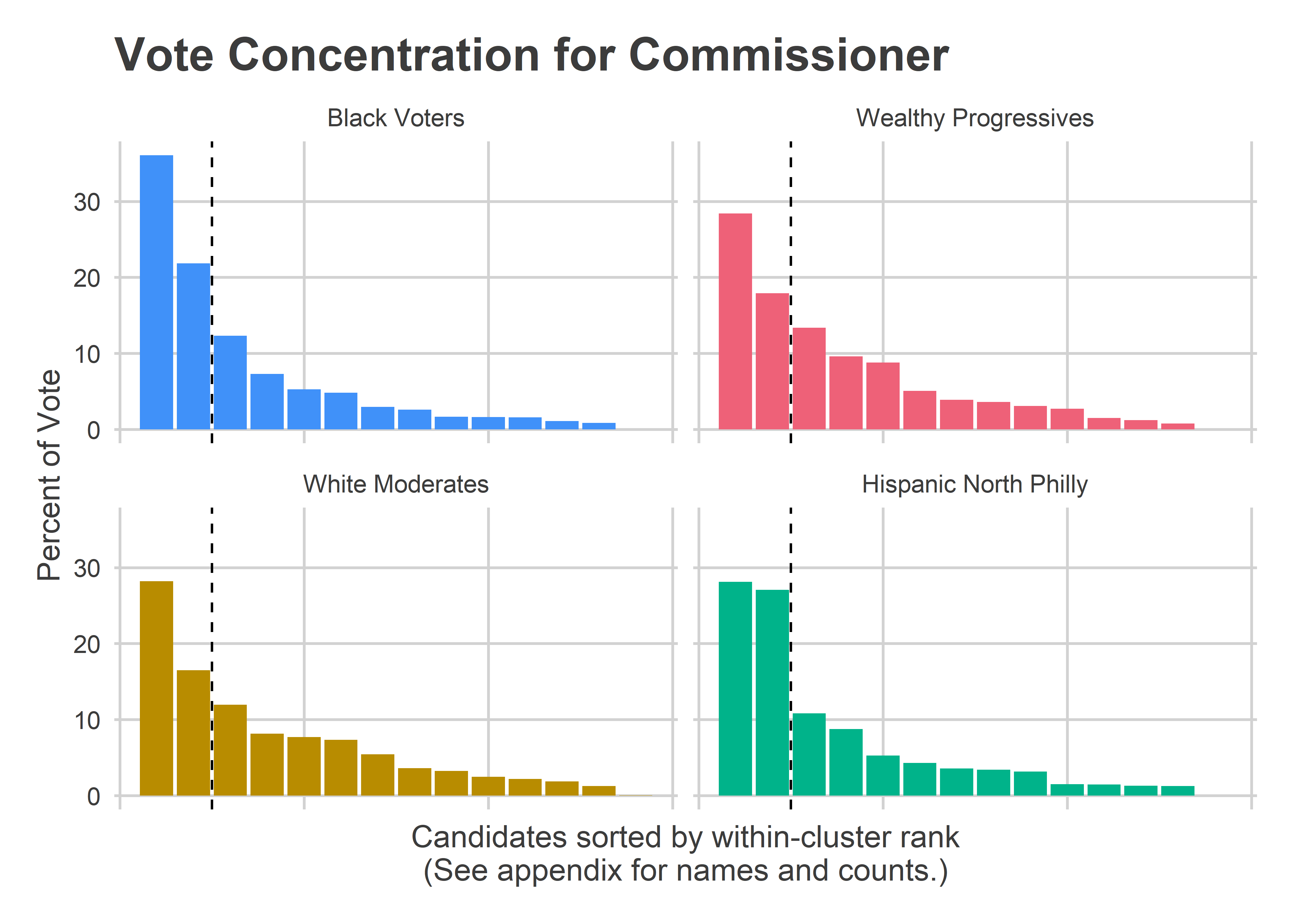
Voters in Black Voter divisions cast 58% of their votes for their two winners, Sabir and Deeley, whereas Wealthy Progressive divisions cast only 46% of their votes for their two, Williams and Devor, and White Moderate divisions only 45%. The fat tail of votes for both the Wealthy Progressives and the White Moderates meant that their favorites received less of a boost.
If Wealthy Progressives had cast their votes for the same ranking of candidates, but using the distribution curve of the Black Voters, then Khalil Williams would have received 6,600 more votes there. This would have been about half of his 12,000 vote city-wide lag.

As I discussed above, it’s not entirely clear that Vote Splitting is the right word for this spreading out of votes. Third and fourth place in the Wealthy Divisions went to Deeley and Sabir, the two winners. So claiming that vote splitting hurt Williams and Devor in these divisions would mean knowing that the votes to the long tail of other candidates would have gone to Williams and Devor, and not Deeley and Sabir.

But Wealthy Progressives did consolidate their vote much more poorly than four years ago. In 2015, Black Voter divisions cast 54% of their vote for their top two commissioners, Wealthy Progressives cast 52%, and White Moderates cast a whopping 58%.

For Common Pleas, the results are exactly the opposite.

View code
# cat_df %>%
#   filter(office == "Common Pleas") %>%
#   group_by(cat) %>%
#   summarise(
#     pvote_winners = sum(pvote * (cat_rank <= 6)),
#     pvote_losers = sum(pvote * (cat_rank > 6))
#   )

get_office_plot("Common Pleas")

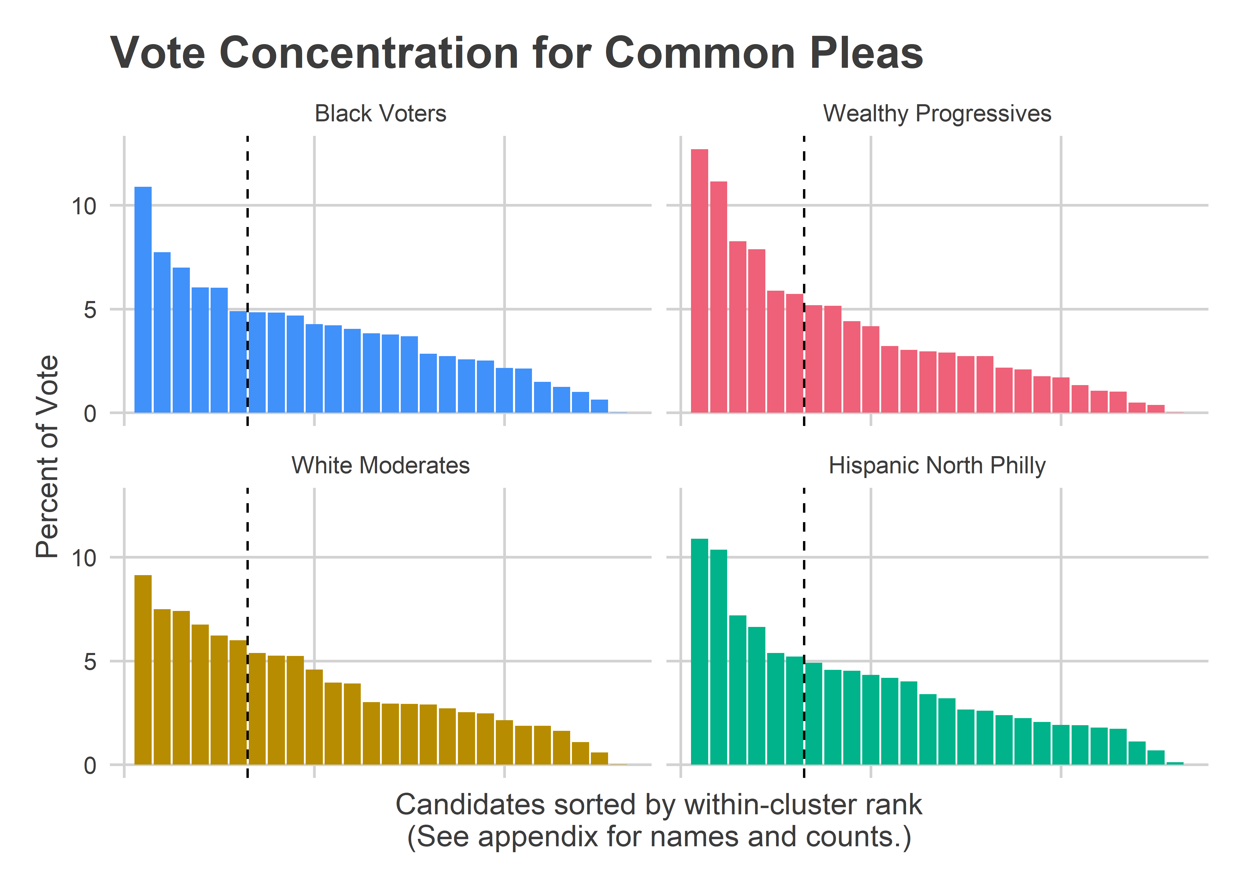
Here, the Black Voters and White Moderates spread out their votes, while the Wealthy Progressive divisions better consolidated their votes to their favored candidates. Those Wealthy Progressives gave 52% of the vote to their cluster winners, and 48% to the rest, while Black Voter and White Moderate divisions only gave 43% to their top six. This concentration of Wealthy Progressive votes is what gave Palmer her dominating win, but it still wasn’t enough for Yu, Barish, and Sias, who were also in the cluster’s top six.

Even with the lower concentration, the sheer vote count power of the Black Voter divisions meant that five of their top six candidates won the city as a whole.

View code
cat_df_15 <- df %>% 
  group_by() %>%
  filter(year == 2015) %>%
  mutate(candidate_name = format_name(CANDIDATE)) %>%
  filter(!is.na(office)) %>%
  left_join(
    divs_svd %>% as.data.frame() %>% select(warddiv, cat)
  ) %>%
  group_by(office, candidate_name, cat) %>%
  summarise(votes = sum(votes)) %>%
  group_by(office, cat) %>%
  mutate(
    pvote = votes/sum(votes),
    cat_rank = rank(desc(votes), ties.method = "first")
  )

# cat_df_15 %>%
#   filter(office == "Council At Large") %>%
#   group_by(cat) %>%
#   summarise(
#     pvote_winner = sum(pvote * (cat_rank == 1)),
#     pvote_winners = sum(pvote * (cat_rank <= 5 & cat_rank > 1)),
#     pvote_losers = sum(pvote * (cat_rank > 5))
#   )
# 
# cat_df_15 %>%
#   filter(office == "Commissioner") %>%
#   group_by(cat) %>%
#   summarise(
#     pvote_winners = sum(pvote * (cat_rank <= 2)),
#     pvote_losers = sum(pvote * (cat_rank > 2))
#   )
# 
# get_office_plot(
#   "Council At Large", cat_df_15, title="Vote Concentration for %s, 2015",
#   show_appendix_text=FALSE
# )
# 
# get_office_plot(
#   "Commissioner", cat_df_15, title="Vote Concentration for %s, 2015",
#   show_appendix_text=FALSE
# )

The effect of vote consolidation

The candidates with support in the Black Voter and White Moderate divisions won out in Council and Commissioner. Common Pleas was less clear. Did vote splitting make the difference?

Yes and no.

In Council, the five winners of the Black Voter clusters won the city as a whole, largely thanks to the sheer number of voters there. The vote consolidation wasn’t terribly different from four years ago.

In Common Pleas, the Wealthy Progressives concentrated their vote more than the others, and won for Palmer and Kyriakakis who had unlucky ballot positions. But the winners of Black Voter divisions also won; it turns out the voting blocs just didn’t disagree all that much.

Commissioner saw the largest consolidation effect. Sabir and Deeley won by dominating the Black Voter and White Moderate divisions, respectively. Williams and Devor, the two Wealthy Progressive division winners, finished third and fourth overall, partially because of a lack of Wealthy Progressive consolidation. Had those divisions concentrated their votes similarly to 2015, Williams and Devor each would have received 1,600 more votes. A sizeable chunk, but not enough to change the election.

Appendix: Cluster Result Tables

View code
format_columns <- function(table, cols, ...){
  for(col in cols){
    table <- table %>% 
      kableExtra::column_spec(column=col, ...)
  }
  return(table)
}
library(knitr)
library(kableExtra)
get_table_for_office <- function(plot_office){
  overall_df <- cat_df %>%
    group_by() %>%
    filter(office == plot_office) %>% 
    group_by(office, candidate_name) %>% 
    summarise(votes = sum(votes)) %>% 
    group_by() %>% 
    mutate(
      cat="Overall", 
      pvote = votes/sum(votes), 
      cat_rank=rank(desc(votes), ties.method = "first")
    )
  
  table <- kable(
    cat_df %>% 
      group_by() %>%
      filter(office == plot_office) %>%
      bind_rows(overall_df) %>%
      mutate(
        cat=factor(cat, levels=c("Overall", names(cat_colors))),
        votes=paste0(scales::comma(votes), " (", round(100 * pvote),"%)")
      ) %>%
      select(candidate_name, cat, votes, cat_rank) %>%
      rename(
        "Rank in Cluster" = cat_rank,
        "Candidate" = candidate_name
      ) %>%
      gather("key", "value", Candidate, votes) %>%
      mutate(key = format_name(key), blank="     ") %>%
      unite(key, cat, key, sep=": ") %>%
      spread(key, value) %>%
      select(
        "Rank in Cluster", 
        blank,
        starts_with("Overall"),
        starts_with("Black"), 
        starts_with("Wealthy"), 
        starts_with("White"), 
        starts_with("Hispanic")
      )
    ,
    caption=sprintf("Cluster Results for %s", plot_office),
    align='l',
    col.names=c("Rank","", rep(c("Candidate", "Votes"), times=5)),
    padding = "4in"
  ) %>%
    column_spec(2, width = "1em") %>% 
    add_header_above(
      c(" " = 2, "Overall" = 2, "Black Voters" = 2, "Wealthy Progressives" = 2,
        "White Moderates" = 2, "Hispanic North Philly" = 2)
    ) %>%
    kable_styling() %>%
    scroll_box(width="100%")
  
  return(table)
}

get_table_for_office("Commissioner")
Cluster Results for Commissioner
Overall
Black Voters
Wealthy Progressives
White Moderates
Hispanic North Philly
Rank Candidate Votes Candidate Votes Candidate Votes Candidate Votes Candidate Votes
1 Omar Sabir 71,303 (24%) Omar Sabir 50,859 (36%) Kahlil Williams 23,546 (28%) Lisa Deeley 16,955 (28%) Omar Sabir 2,559 (28%)
2 Lisa Deeley 61,278 (21%) Lisa Deeley 30,766 (22%) Jen Devor 14,853 (18%) Omar Sabir 9,909 (16%) Lisa Deeley 2,465 (27%)
3 Kahlil Williams 48,884 (17%) Kahlil Williams 17,346 (12%) Lisa Deeley 11,092 (13%) Kahlil Williams 7,193 (12%) Marwan Kreidie 984 (11%)
4 Jen Devor 23,752 (8%) Marwan Kreidie 10,295 (7%) Omar Sabir 7,976 (10%) Jen Devor 4,905 (8%) Kahlil Williams 799 (9%)
5 Marwan Kreidie 23,190 (8%) Annette Thompson 7,422 (5%) Marwan Kreidie 7,278 (9%) Marwan Kreidie 4,633 (8%) Annette Thompson 480 (5%)
6 Annette Thompson 14,389 (5%) Dennis Lee 6,828 (5%) Luigi Borda 4,210 (5%) Luigi Borda 4,422 (7%) Luigi Borda 390 (4%)
7 Dennis Lee 11,649 (4%) Carla Cain 4,161 (3%) Annette Thompson 3,217 (4%) Annette Thompson 3,270 (5%) Jen Devor 325 (4%)
8 Luigi Borda 11,352 (4%) Jen Devor 3,669 (3%) Carla Cain 3,004 (4%) Carla Cain 2,160 (4%) Dennis Lee 309 (3%)
9 Carla Cain 9,613 (3%) Luigi Borda 2,330 (2%) Dennis Lee 2,558 (3%) Dennis Lee 1,954 (3%) Carla Cain 288 (3%)
10 Moira Bohannon 5,054 (2%) Lewis Harris Jr 2,292 (2%) Moira Bohannon 2,247 (3%) Moira Bohannon 1,485 (2%) Robin Trent 136 (1%)
11 Robin Trent 4,949 (2%) Robin Trent 2,239 (2%) Robin Trent 1,259 (2%) Robin Trent 1,315 (2%) Moira Bohannon 133 (1%)
12 Warren Bloom 3,808 (1%) Warren Bloom 1,563 (1%) Warren Bloom 1,001 (1%) Warren Bloom 1,124 (2%) Warren Bloom 120 (1%)
13 Lewis Harris Jr 3,793 (1%) Moira Bohannon 1,189 (1%) Lewis Harris Jr 627 (1%) Lewis Harris Jr 758 (1%) Lewis Harris Jr 116 (1%)
14 Write In 34 (0%) Write In 10 (0%) Write In 4 (0%) Write In 19 (0%) Write In 1 (0%)
View code
get_table_for_office("Council At Large")
Cluster Results for Council At Large
Overall
Black Voters
Wealthy Progressives
White Moderates
Hispanic North Philly
Rank Candidate Votes Candidate Votes Candidate Votes Candidate Votes Candidate Votes
1 Helen Gym 108,604 (16%) Helen Gym 47,309 (15%) Helen Gym 37,687 (18%) Helen Gym 21,087 (15%) Helen Gym 2,521 (14%)
2 Allan Domb 67,193 (10%) Isaiah Thomas 37,294 (12%) Justin Diberardinis 22,895 (11%) Allan Domb 15,403 (11%) Allan Domb 1,747 (9%)
3 Isaiah Thomas 64,045 (10%) Allan Domb 33,664 (11%) Erika Almirón 18,618 (9%) Justin Diberardinis 10,190 (7%) Adrián Rivera-Reyes 1,720 (9%)
4 Derek S Green 61,070 (9%) Derek S Green 33,145 (11%) Eryn Santamoor 17,209 (8%) Isaiah Thomas 10,173 (7%) Isaiah Thomas 1,576 (8%)
5 Katherine Gilmore Richardson 45,470 (7%) Katherine Gilmore Richardson 24,581 (8%) Derek S Green 17,085 (8%) Derek S Green 9,496 (7%) Deja Lynn Alvarez 1,359 (7%)
6 Justin Diberardinis 42,643 (6%) Adrián Rivera-Reyes 16,323 (5%) Allan Domb 16,379 (8%) Katherine Gilmore Richardson 9,396 (7%) Derek S Green 1,344 (7%)
7 Adrián Rivera-Reyes 35,565 (5%) Deja Lynn Alvarez 12,638 (4%) Isaiah Thomas 15,002 (7%) Eryn Santamoor 8,084 (6%) Katherine Gilmore Richardson 1,232 (7%)
8 Eryn Santamoor 35,026 (5%) Sandra Dungee Glenn 11,153 (4%) Adrián Rivera-Reyes 10,545 (5%) Adrián Rivera-Reyes 6,977 (5%) Justin Diberardinis 899 (5%)
9 Erika Almirón 34,329 (5%) Eryn Santamoor 9,129 (3%) Katherine Gilmore Richardson 10,261 (5%) Erika Almirón 6,254 (5%) Erika Almirón 715 (4%)
10 Deja Lynn Alvarez 26,617 (4%) Erika Almirón 8,742 (3%) Deja Lynn Alvarez 7,190 (3%) Deja Lynn Alvarez 5,430 (4%) Eryn Santamoor 604 (3%)
11 Sandra Dungee Glenn 18,105 (3%) Justin Diberardinis 8,659 (3%) Ethelind Baylor 5,646 (3%) Beth Finn 4,333 (3%) Ogbonna Paul Hagins 576 (3%)
12 Ethelind Baylor 14,259 (2%) Ogbonna Paul Hagins 7,260 (2%) Beth Finn 5,281 (3%) Joseph A Diorio 3,186 (2%) Fernando Treviño 530 (3%)
13 Beth Finn 14,015 (2%) Fareed Abdullah 7,170 (2%) Fernando Treviño 4,519 (2%) Ethelind Baylor 2,808 (2%) Beth Finn 389 (2%)
14 Ogbonna Paul Hagins 12,570 (2%) Asa Khalif 5,682 (2%) Sandra Dungee Glenn 3,795 (2%) Fernando Treviño 2,799 (2%) Sandra Dungee Glenn 379 (2%)
15 Fernando Treviño 11,646 (2%) Ethelind Baylor 5,535 (2%) Ogbonna Paul Hagins 2,369 (1%) Sandra Dungee Glenn 2,778 (2%) Joseph A Diorio 358 (2%)
16 Fareed Abdullah 10,676 (2%) Latrice Y Bryant 5,473 (2%) Asa Khalif 2,303 (1%) Ogbonna Paul Hagins 2,365 (2%) Billy Thompson 306 (2%)
17 Asa Khalif 9,779 (1%) Billy Thompson 5,300 (2%) Fareed Abdullah 1,821 (1%) Billy Thompson 2,205 (2%) Ethelind Baylor 270 (1%)
18 Billy Thompson 9,166 (1%) Beth Finn 4,012 (1%) Latrice Y Bryant 1,773 (1%) Vinny Black 1,801 (1%) Edwin Santana 269 (1%)
19 Latrice Y Bryant 8,966 (1%) Fernando Treviño 3,798 (1%) Hena Veit 1,413 (1%) Hena Veit 1,620 (1%) Latrice Y Bryant 269 (1%)
20 Joseph A Diorio 7,803 (1%) Edwin Santana 3,061 (1%) Billy Thompson 1,355 (1%) Asa Khalif 1,538 (1%) Fareed Abdullah 258 (1%)
21 Hena Veit 5,474 (1%) Joseph A Diorio 3,054 (1%) Joseph A Diorio 1,205 (1%) Latrice Y Bryant 1,451 (1%) Asa Khalif 256 (1%)
22 Edwin Santana 5,272 (1%) Wayne Allen 2,926 (1%) Wayne Allen 958 (0%) Fareed Abdullah 1,427 (1%) Hena Veit 232 (1%)
23 Wayne Allen 4,941 (1%) Hena Veit 2,209 (1%) Edwin Santana 883 (0%) Bobbie Curry 1,255 (1%) Vinny Black 168 (1%)
24 Vinny Black 4,516 (1%) Mark Ross 2,137 (1%) Mark Ross 722 (0%) Mark Ross 1,253 (1%) Wayne Allen 158 (1%)
25 Mark Ross 4,255 (1%) Bobbie Curry 1,923 (1%) Vinny Black 685 (0%) Edwin Santana 1,059 (1%) Bobbie Curry 146 (1%)
26 Bobbie Curry 3,920 (1%) Vinny Black 1,862 (1%) Bobbie Curry 596 (0%) Wayne Allen 899 (1%) Mark Ross 143 (1%)
27 Devon Cade 2,854 (0%) Wayne Edmund Dorsey 1,606 (1%) Devon Cade 522 (0%) Devon Cade 683 (0%) Devon Cade 116 (1%)
28 Wayne Edmund Dorsey 2,780 (0%) Devon Cade 1,533 (0%) Wayne Edmund Dorsey 428 (0%) Wayne Edmund Dorsey 643 (0%) Wayne Edmund Dorsey 103 (1%)
29 Write In 316 (0%) Write In 127 (0%) Write In 101 (0%) Write In 77 (0%) Write In 11 (0%)
View code
get_table_for_office("Common Pleas")
Cluster Results for Common Pleas
Overall
Black Voters
Wealthy Progressives
White Moderates
Hispanic North Philly
Rank Candidate Votes Candidate Votes Candidate Votes Candidate Votes Candidate Votes
1 Jennifer Schultz 59,547 (8%) Joshua Roberts 35,820 (11%) Tiffany Palmer 29,310 (13%) Jennifer Schultz 13,789 (9%) Joshua Roberts 2,281 (11%)
2 Anthony Kyriakakis 58,128 (8%) Jennifer Schultz 25,424 (8%) Anthony Kyriakakis 25,711 (11%) Joshua Roberts 11,317 (7%) Jennifer Schultz 2,171 (10%)
3 Joshua Roberts 55,702 (8%) Carmella Jacquinto 23,005 (7%) Kay Yu 19,046 (8%) Anthony Kyriakakis 11,187 (7%) Carmella Jacquinto 1,506 (7%)
4 Tiffany Palmer 55,586 (8%) Anthony Kyriakakis 19,840 (6%) Jennifer Schultz 18,163 (8%) James C Crumlish 10,203 (7%) Anthony Kyriakakis 1,390 (7%)
5 James C Crumlish 39,217 (5%) Cateria R McCabe 19,788 (6%) Wendi Barish 13,562 (6%) Tiffany Palmer 9,392 (6%) Craig Levin 1,127 (5%)
6 Carmella Jacquinto 38,920 (5%) James C Crumlish 16,107 (5%) Henry McGregor Sias 13,202 (6%) Wendi Barish 9,062 (6%) Wendi Barish 1,092 (5%)
7 Wendi Barish 36,998 (5%) Tiffany Palmer 15,927 (5%) Chris Hall 11,956 (5%) Carmella Jacquinto 8,128 (5%) James C Crumlish 1,030 (5%)
8 Cateria R McCabe 36,214 (5%) Craig Levin 15,872 (5%) James C Crumlish 11,877 (5%) Beth Grossman 7,932 (5%) Tiffany Palmer 957 (5%)
9 Kay Yu 34,475 (5%) Henry McGregor Sias 15,413 (5%) Nicola Serianni 10,173 (4%) Nicola Serianni 7,923 (5%) Jon Marshall 948 (5%)
10 Henry McGregor Sias 33,560 (5%) Leon Goodman 14,027 (4%) Cateria R McCabe 9,629 (4%) Craig Levin 6,916 (5%) Nicola Serianni 907 (4%)
11 Craig Levin 30,746 (4%) Sherman Toppin 13,854 (4%) Leon Goodman 7,394 (3%) Kay Yu 5,979 (4%) Cateria R McCabe 877 (4%)
12 Nicola Serianni 28,328 (4%) Wendi Barish 13,282 (4%) Beth Grossman 6,965 (3%) Cateria R McCabe 5,920 (4%) Henry McGregor Sias 841 (4%)
13 Leon Goodman 26,352 (4%) Kendra McCrae 12,585 (4%) Craig Levin 6,831 (3%) Chris Hall 4,552 (3%) Beth Grossman 711 (3%)
14 Chris Hall 23,891 (3%) Terri M Booker 12,388 (4%) Vicki Markovitz 6,677 (3%) Vicki Markovitz 4,445 (3%) Sherman Toppin 671 (3%)
15 Beth Grossman 23,876 (3%) Jon Marshall 12,105 (4%) Joshua Roberts 6,284 (3%) James F Berardinelli 4,412 (3%) Leon Goodman 556 (3%)
16 Kendra McCrae 21,853 (3%) Nicola Serianni 9,325 (3%) Carmella Jacquinto 6,281 (3%) Leon Goodman 4,375 (3%) Kendra McCrae 545 (3%)
17 Sherman Toppin 19,331 (3%) Kay Yu 8,950 (3%) Kendra McCrae 4,999 (2%) Henry McGregor Sias 4,104 (3%) Kay Yu 500 (2%)
18 Jon Marshall 19,322 (3%) Laurie Dow 8,464 (3%) James F Berardinelli 4,792 (2%) Jon Marshall 3,823 (3%) Terri M Booker 470 (2%)
19 Terri M Booker 18,750 (3%) Beth Grossman 8,268 (3%) Janine D Momasso 4,052 (2%) Kendra McCrae 3,724 (2%) Vicki Markovitz 431 (2%)
20 Vicki Markovitz 16,433 (2%) Janine D Momasso 7,111 (2%) Laurie Dow 3,924 (2%) Laurie Dow 3,233 (2%) Janine D Momasso 402 (2%)
21 Laurie Dow 16,020 (2%) Chris Hall 7,009 (2%) Terri M Booker 3,061 (1%) Terri M Booker 2,831 (2%) Laurie Dow 399 (2%)
22 Janine D Momasso 14,384 (2%) Vicki Markovitz 4,880 (1%) Jon Marshall 2,446 (1%) Janine D Momasso 2,819 (2%) Chris Hall 374 (2%)
23 James F Berardinelli 13,663 (2%) James F Berardinelli 4,098 (1%) Sherman Toppin 2,355 (1%) Sherman Toppin 2,451 (2%) James F Berardinelli 361 (2%)
24 Robert Trimble 6,305 (1%) Robert Trimble 3,300 (1%) Robert Trimble 1,123 (0%) Robert Trimble 1,649 (1%) Robert Trimble 233 (1%)
25 Gregory Weyer 3,962 (1%) Gregory Weyer 2,069 (1%) Gregory Weyer 861 (0%) Gregory Weyer 889 (1%) Gregory Weyer 143 (1%)
26 Write In 108 (0%) Write In 33 (0%) Write In 23 (0%) Write In 27 (0%) Write In 25 (0%)