Covid-19 and PA’s first-ever mail-in ballot election.
With Coronavirus upon us, Philadelphians are re-evaluating how we might vote in the June 2nd Primary. Coincidentally, this is also the first year that Pennsylvanians can request mail-in ballots even if they won’t be absentee. This combination has led to a huge amount of requests, and big questions about what this might mean for turnout and the results.
The friendly folks at the Commissioners’ Office have sent me all of Philadelphia’s requests through Thursday May 7th. Let’s dig in.
An astounding 91,587 voters have requested ballots. Philadelphia has 913,000 active registered voters. In the 2019 Primary, 217,000 people voted. For a brand new program, that number is a huge percent.
Who is requesting ballots?
As with everything political in this city, that pattern wasn’t equal across the city.
View code
library(tidyr)
library(dplyr)
library(readr)
library(ggplot2)
library(sf)
library(magrittr)
library(lubridate)
setwd("C:/Users/Jonathan Tannen/Dropbox/sixty_six/posts/mail_in/")
source("../../admin_scripts/util.R")
fve <- readRDS("../../data/processed_data/voter_db/fve.Rds")
v2e <- readRDS("../../data/processed_data/voter_db/voters_to_elections.Rds")
elections <- readRDS("../../data/processed_data/voter_db/elections.Rds")
mail_in <- read_csv("../../data/voter_registration/mail_in/Absentee_Mail-in Ballot Listing (5-7-20).csv")
mail_in %<>% filter(!duplicated(`ID Number`))
mail_in %<>% left_join(fve, by=c("ID Number" = "voter_id"))
# table(mail_in$voter_status, useNA = "always")
divs <- st_read("../../data/gis/warddivs/201911/Political_Divisions.shp")divs %<>% mutate(warddiv = pretty_div(DIVISION_N))
mail_in_div <- mail_in %>%
group_by(warddiv) %>%
summarise(n_mail = n())
fve_div <- fve %>%
filter(voter_status == "A") %>%
group_by(warddiv) %>%
summarise(n_reg = n())
df_major <- readRDS("../../data/processed_data/df_major_20191203.Rds")
df_major %<>% mutate(warddiv = pretty_div(warddiv))
turnout <- df_major %>%
filter(is_topline_office) %>%
group_by(warddiv, year, election) %>%
summarise(turnout = sum(votes))
turnout_wide <- turnout %>%
unite("key", year, election) %>%
spread(key, turnout)
divs %<>% left_join(mail_in_div) %>% mutate(n_mail = ifelse(is.na(n_mail), 0, n_mail))
divs %<>% left_join(fve_div)
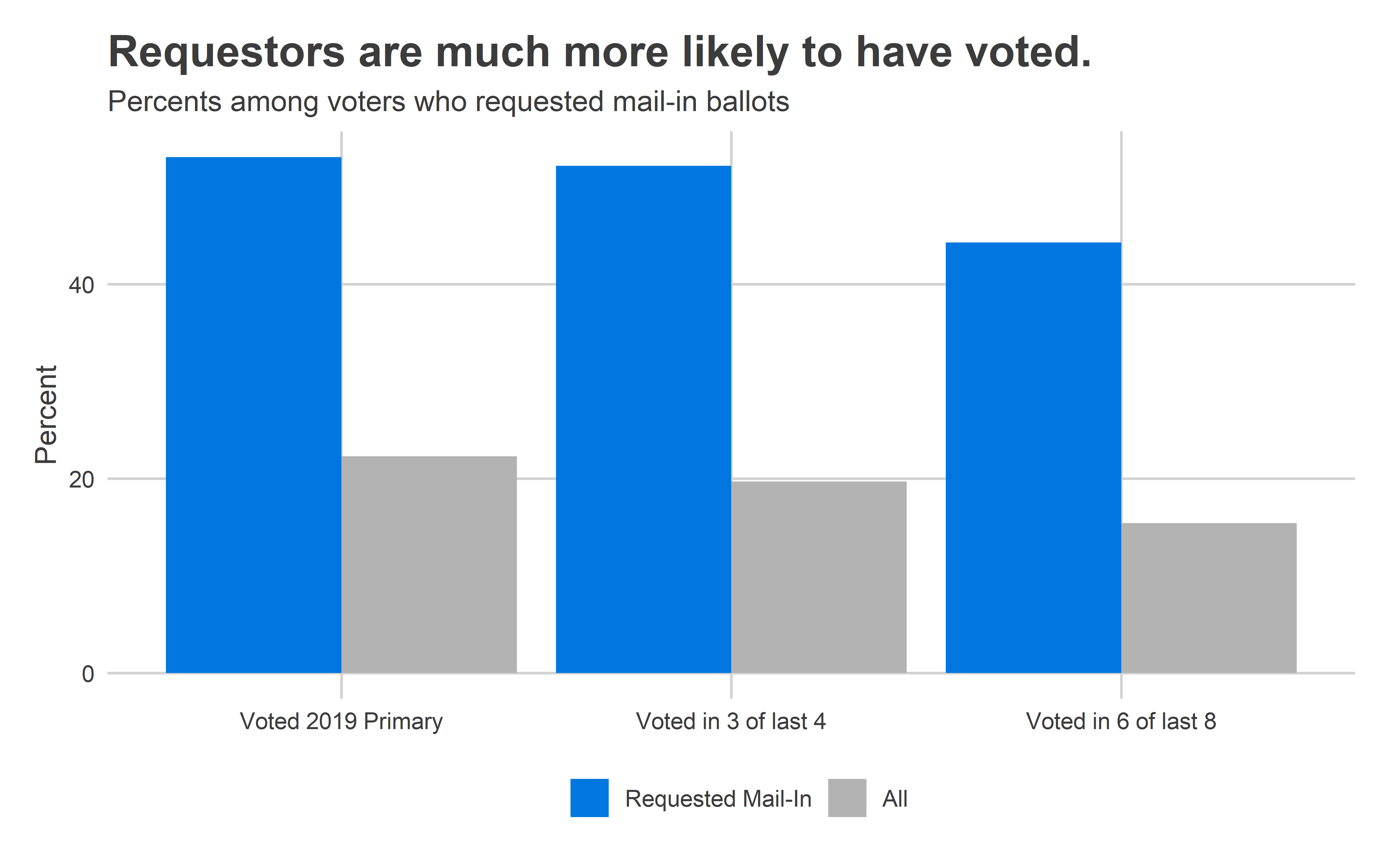
divs %<>% left_join(turnout_wide)These requestors are much more likely to have voted than a typical Philadelphian. A whopping 53% of them voted in the 2019 Primary (overall turnout among active voters was 24%). Some 52% of them voted in at least three of the last four elections, and 44% in six of the last eight (the number is presumably lower because of people who didn’t live in the state eight years ago).
View code
mail_in_v2e <- v2e %>%
  mutate(mail_in_reqd = voter_id %in% mail_in$`ID Number`) %>%
  inner_join(
    elections %>% filter(is_general | is_primary, year >= 2016) %>%
      select(election_date, year, fve_election_id)
  ) %>%
  group_by(voter_id, mail_in_reqd) %>%
  summarise(
    voted_2019 = !is.na(vote_method[election_date == "2019-05-21"]),
    voted_l4 = sum(!is.na(vote_method[year >= 2018])),
    voted_l8 = sum(!is.na(vote_method)),
    cnt = n()
  ) %>%
  group_by(mail_in_reqd) %>%
  summarise(
    voted_2019 = sum(voted_2019),
    voted_l4 = sum(voted_l4 >= 3),
    voted_l8 = sum(voted_l8 >= 6),
    cnt = n()
  )

mail_in_v2e <- bind_rows(
  mail_in_v2e %>% mutate(mail_in_reqd = ifelse(mail_in_reqd, "Requested Mail-In", "No Request")),
  mail_in_v2e %>% mutate(mail_in_reqd = "All") %>% group_by(mail_in_reqd) %>% summarise_all(sum)
)

ggplot(
  mail_in_v2e %>% filter(mail_in_reqd %in% c("Requested Mail-In", "All")) %>%
    mutate(mail_in_reqd = forcats::fct_inorder(mail_in_reqd)) %>%
    gather("key", "value", voted_2019, voted_l4, voted_l8) %>%
    mutate(
      key = case_when(
        key == "voted_2019" ~ "Voted 2019 Primary",
        key == "voted_l4" ~ "Voted in 3 of last 4",
        key == "voted_l8" ~ "Voted in 6 of last 8"
      )
    ),
  aes(x=key, y=100*value / cnt, fill=mail_in_reqd)
) +
  geom_bar(stat="identity", position="dodge") +
  theme_sixtysix() +
  scale_fill_manual(values = c(strong_blue, grey(0.70))) +
  labs(
    x = NULL,
    y = "Percent",
    fill = NULL,
    title = "Requestors are much more likely to have voted.",
    subtitle = "Percents among voters who requested mail-in ballots"
  )
By Age
The mail-in requests are coming disproportionately from younger voters. The cohort aged 30-40 made up only 15% of votes in the 2019 Primary, but over 23% of the requests so far.
View code
age_cuts <- c(18, seq(10, 120, 10))
fve_age <- fve %>%
  filter(voter_status == "A") %>%
  mutate(
    age = (lubridate::ymd("2020-06-02") - lubridate::ymd(dob)) / dyears(1),
    age_cat = cut(age, age_cuts)
  ) %>%
  group_by(age_cat) %>%
  summarise(n = n()) %>%
  ungroup() %>%
  mutate(prop = n / sum(n))

fve_age_2019 <- fve %>%
  inner_join(
    v2e %>%
      inner_join(elections %>% filter(election_date == "2019-05-21")) %>%
      filter(!is.na(vote_method))
  ) %>%
  mutate(
    age = (lubridate::ymd("2020-06-02") - lubridate::ymd(dob)) / dyears(1),
    age_cat = cut(age, age_cuts)
  ) %>%
  group_by(age_cat) %>%
  summarise(n = n()) %>%
  ungroup() %>%
  mutate(prop = n / sum(n))

mail_in_age <- mail_in %>%
  mutate(
    age = (lubridate::ymd("2020-06-02") - lubridate::ymd(dob)) / dyears(1),
    age_cat = cut(age, age_cuts)
  ) %>%
  group_by(age_cat) %>%
  summarise(n = n()) %>%
  ungroup() %>%
  mutate(prop = n / sum(n))

age_cats <- bind_rows(
  mail_in_age %>% mutate(source = "Mail-In Requests"),
  fve_age_2019 %>% mutate(source = "2019 Primary Voters"),
  fve_age %>% mutate(source = "Active Registered Voters")
) %>%
  mutate(source = forcats::fct_inorder(source))


ggplot(
  age_cats %>%
    filter(!is.na(age_cat), !age_cat %in% c("(0,10]","(100,110]","(110,120]")) %>%
    mutate(
      age_cat = droplevels(age_cat)
    ),
  aes(x = age_cat, y = 100 * prop, fill=source)
) + geom_bar(
  stat="identity",
  position="dodge"
) +
  theme_sixtysix() +
  labs(
    y="Percent of Total",
    x = "Age",
    fill = ""
  ) +
  scale_fill_manual(values = c(strong_blue, grey(0.70), grey(0.9))) +
  ggtitle("Voters under 40 are disproportionately requesting ballots")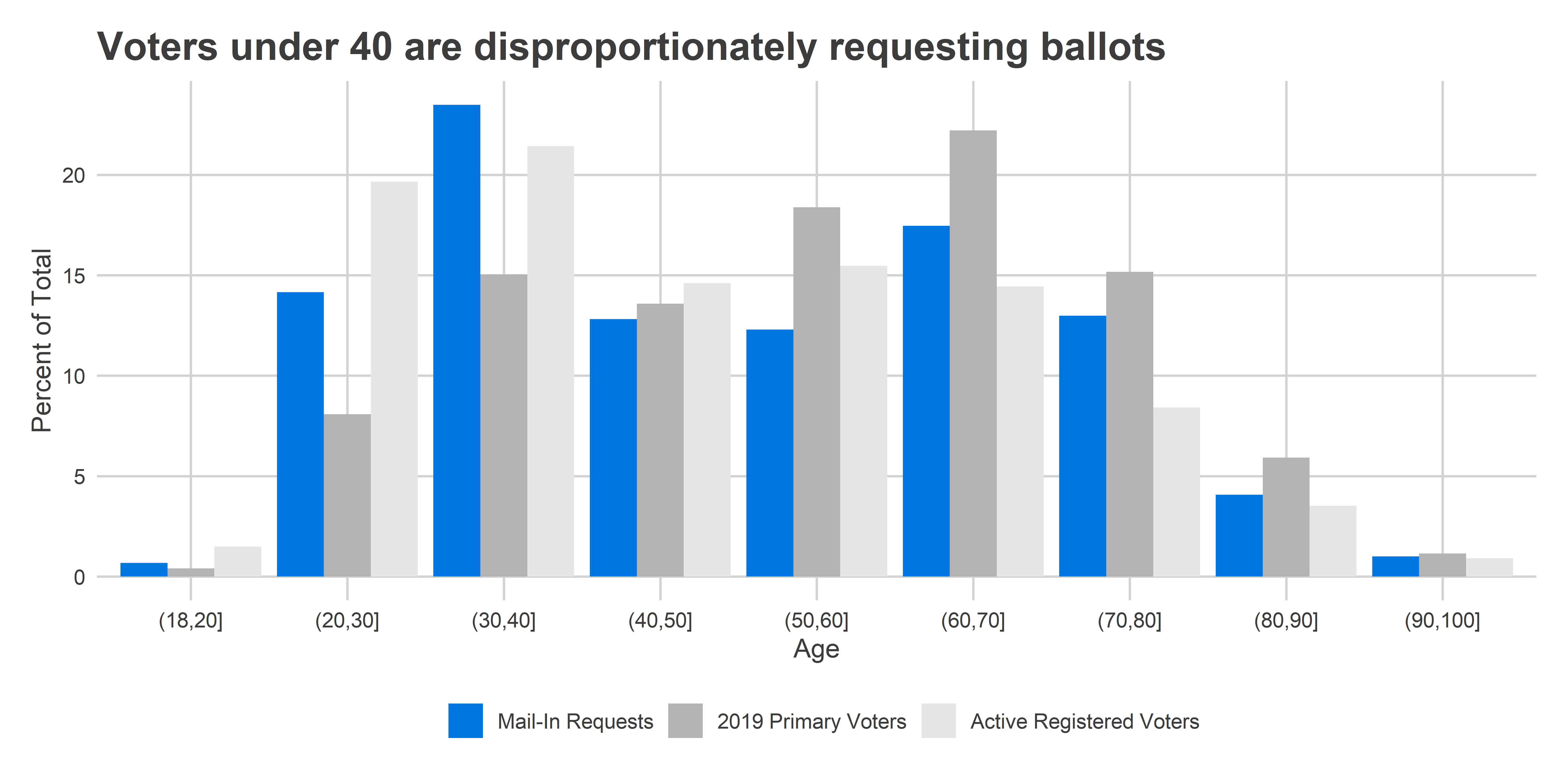
By Neighborhood
Geographically, the patterns are even starker. More than 13,000 of the requests came from the two Center City wards–5 and 8–alone.
[See the Appendix for Division-level maps.]
View code
library(leaflet)

make_leaflet <- function(
  sf,
  color_col,
  title,
  is_percent=FALSE,
  pal="viridis"
){
  zoom <- 11

  min_value <- min(sf[[color_col]], na.rm=TRUE)
  max_value <- max(sf[[color_col]], na.rm=TRUE)

  sigfig <- round(log10(max_value-min_value)) - 1
  step_size <- 2 * 10^(sigfig)

  min_value <- step_size * (min_value %/% step_size)
  max_value <- step_size * (max_value %/% step_size + 1)

  color_numeric <- colorNumeric(
    pal,
    domain=c(min_value, max_value)
  )

  legend_values <- seq(min_value, max_value, step_size)
  legend_colors <- color_numeric(legend_values)
  if(is_percent){
    legend_labels <- sprintf("%s%%", legend_values)
  } else{
    legend_labels <- scales::comma(legend_values)
  }

  bbox <- st_bbox(sf)

  leaflet(
    options=leafletOptions(
      minZoom=zoom,
      # maxZoom=zoom,
      zoomControl=TRUE
      # dragging=FALSE
    )
  )%>%
    addProviderTiles(providers$Stamen.TonerLite) %>%
    addPolygons(
      data=sf$geometry,
      weight=0,
      color="white",
      opacity=1,
      fillOpacity = 0.8,
      smoothFactor = 0,
      fillColor = color_numeric(sf[[color_col]]),
      popup=sf$popup
    ) %>%
    setMaxBounds(
      lng1=bbox["xmin"],
      lng2=bbox["xmax"],
      lat1=bbox["ymin"],
      lat2=bbox["ymax"]
    ) %>%
    addControl(title, position="topright", layerId="map_title") %>%
    addLegend(
      layerId="geom_legend",
      position="bottomright",
      colors=legend_colors,
      labels=legend_labels
    )
}

wards <- divs %>%
  mutate(ward = substr(warddiv, 1, 2)) %>%
  group_by(ward) %>%
  summarise_at(
    .funs=list(sum),
    .vars=vars(n_mail, n_reg, `2002_general`:`2019_primary`)
  )

wards %<>%
  mutate(
    popup = sprintf(
      paste(
        c(
          "<b>Ward %s</b>",
          "Active Registered Voters: %s",
          "Mail-In Requests: %s",
          "Votes in the 2019 Primary: %s",
          "Votes in the 2016 Primary: %s"
        ),
        collapse = "<br>"
      ),
      ward,
      scales::comma(n_reg),
      scales::comma(n_mail),
      scales::comma(round(`2019_primary`)),
      scales::comma(round(`2016_primary`))
    )
  )

wards$color_mail <- wards$n_mail
wards_mail <- make_leaflet(
  wards,
  "color_mail",
  "Number of Mail-In Requests"
)
library(widgetframe)
knitr::opts_chunk$set(widgetframe_self_contained = TRUE)
frameWidget(wards_mail)
As a percent of all voters, Center City, the wealthy ring around it, and Mount Airy/Chestnut Hill stand out. These Wards make up what I’ve dubbed the Wealthy Progressives.
View code
wards$color_mail_vs_reg <- 100 * wards$n_mail / wards$n_reg
mail_reg <- make_leaflet(
  wards,
  "color_mail_vs_reg",
  "Mail-In Requests as % of Active Registered Voters",
  is_percent=TRUE
)
knitr::opts_chunk$set(widgetframe_self_contained = TRUE)
frameWidget(mail_reg)
View code
wards$color_mail_vs_2019 <- 100 * wards$n_mail / wards$`2019_primary`
mail_2019 <- make_leaflet(
  wards,
  "color_mail_vs_2019",
  "Mail-in requests as % of 2019 Primary voters",
  is_percent=TRUE
)
knitr::opts_chunk$set(widgetframe_self_contained = TRUE)
frameWidget(mail_2019)
In fact, aggregating by those Division Cohorts paints a stark picture.
View code
div_cats <- readRDS("../../data/processed_data/div_cats_20200411.RDS")
divs %<>% left_join(div_cats %>% select(warddiv, cat))
cat_colors <- c(
  "Black Voters" = light_blue,
  "Wealthy Progressives" = light_red,
  "White Moderates" = light_orange,
  "Hispanic North Philly" = light_green
)

div_cats <- divs %>%
  as.data.frame() %>%
  select(-geometry) %>%
  group_by(cat) %>%
  summarise_at(
    .funs=list(sum),
    .vars=vars(n_mail, n_reg, `2002_general`:`2019_primary`)
  ) %>%
  ungroup()

ggplot(
  div_cats,
  aes(x = cat, y = n_reg, fill=cat)
) + geom_bar(
  stat="identity",
  position="dodge"
) +
  theme_sixtysix() + # %+replace% theme(axis.text.x = element_blank())+
  scale_y_continuous(labels=scales::comma) +
  labs(
    y=NULL,
    x = NULL,
    fill = "",
    title="Black Voter Divisions represent nearly half of Active Voters",
    subtitle="Active Registered Voters"
  ) +
  scale_fill_manual(values = cat_colors, guide=FALSE)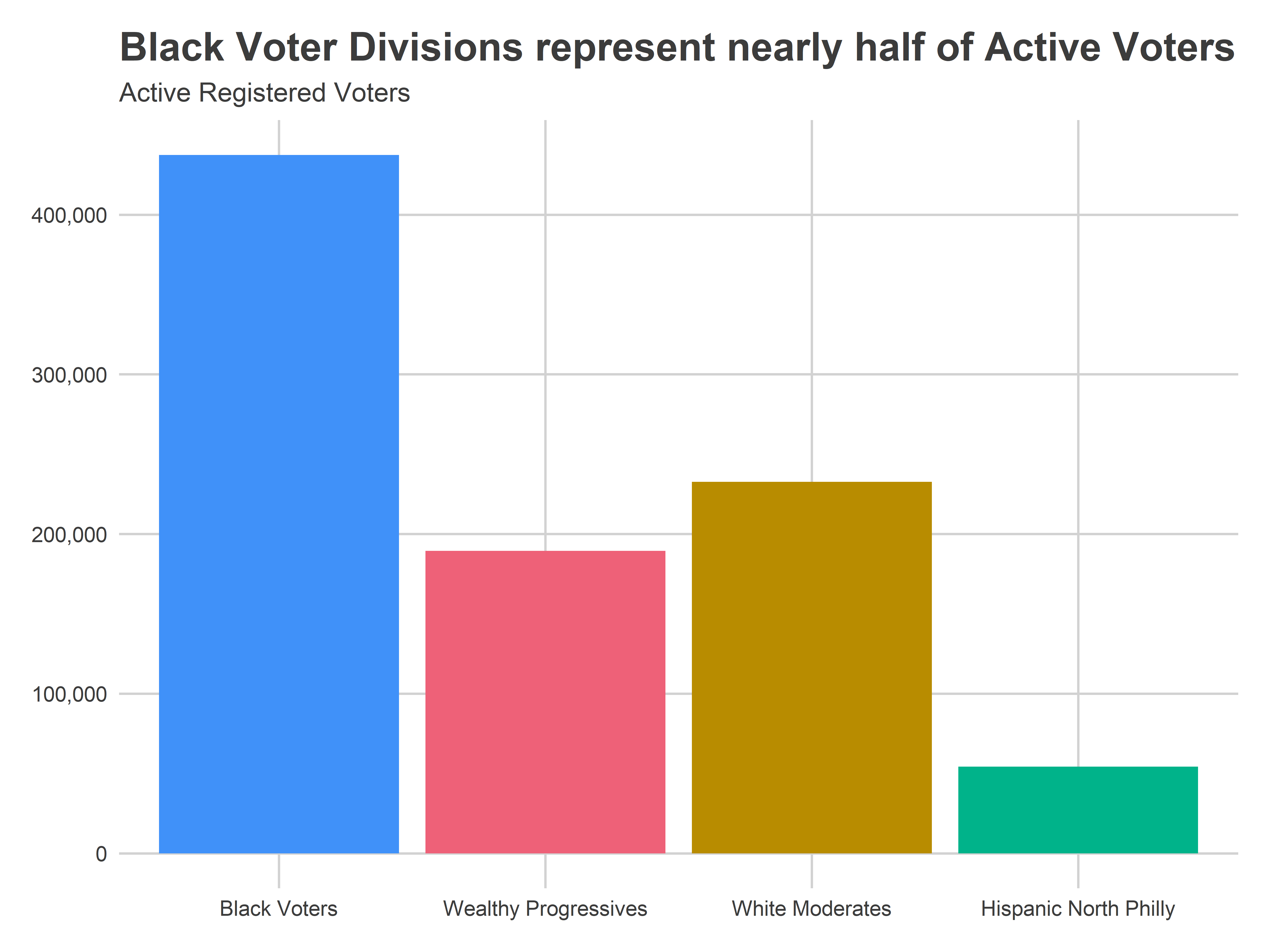
View code
ggplot(
  div_cats %>%
    mutate(prop_mail = n_mail / n_reg),
  aes(x = cat, y = 100 * prop_mail, fill=cat)
) + geom_bar(
  stat="identity",
  position="dodge"
) +
  theme_sixtysix() %+replace% theme(title = element_text(size = 10)) +
  labs(
    y=NULL,
    x = NULL,
    fill = "",
    title="But Wealthy Progressive Divisions have the most mail-in requests",
    subtitle="Mail-in requests as a percent of active registered voters"
  ) +
  scale_fill_manual(values = cat_colors, guide=FALSE)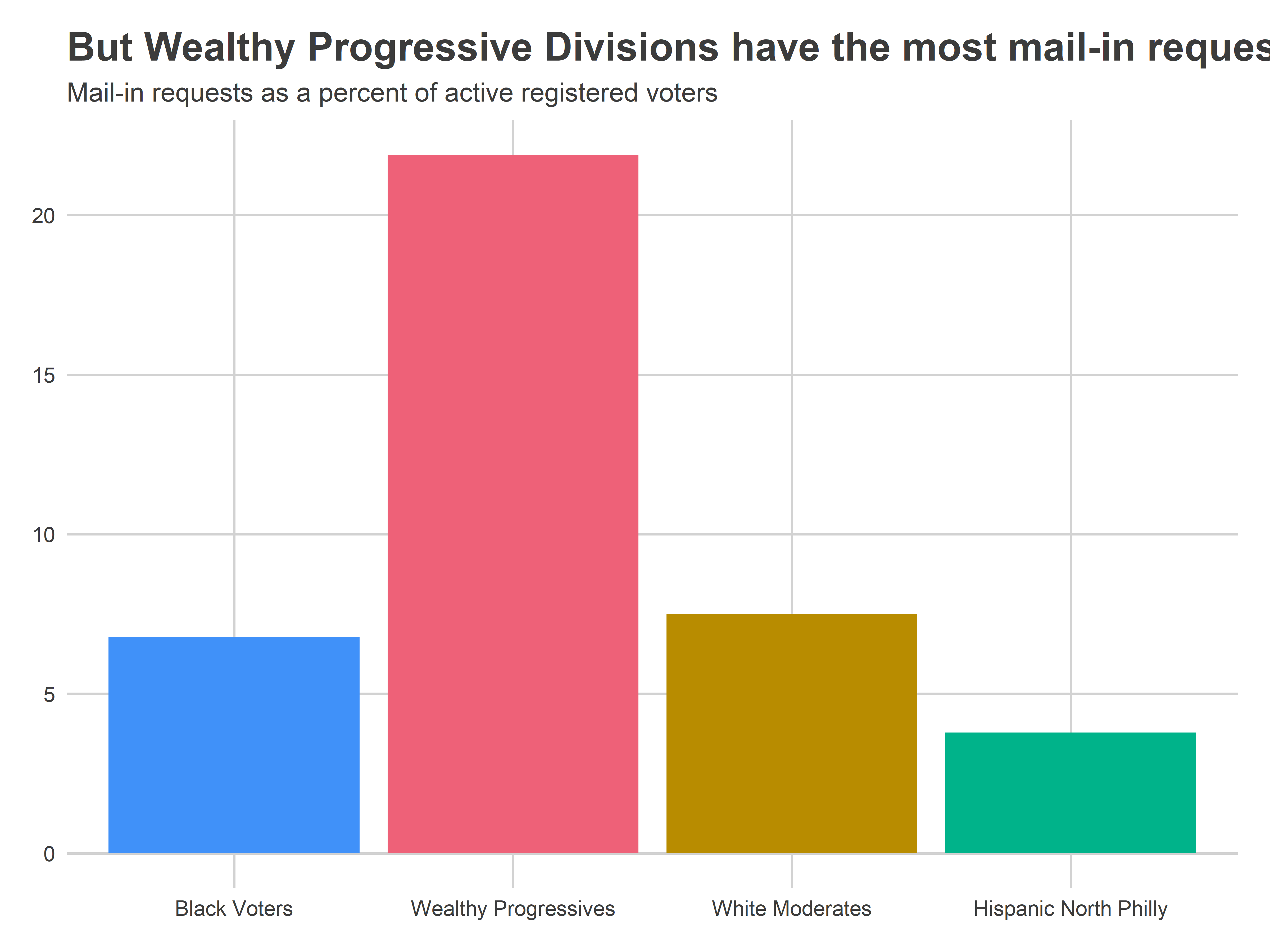
View code
ggplot(
  div_cats %>%
    mutate(prop_2019 = n_mail / `2019_primary`),
  aes(x = cat, y = 100 * prop_2019, fill=cat)
) + geom_bar(
  stat="identity",
  position="dodge"
) +
  theme_sixtysix() + # %+replace% theme(axis.text.x = element_blank())+
  labs(
    y=NULL,
    x = NULL,
    fill = "",
    title="Mail-in requests as percent of 2019 Primary turnout",
    subtitle="Requests from Wealthy Progressive Divisions are nearly 80% of their 2019 turnout."
  ) +
  scale_fill_manual(values = cat_colors, guide=FALSE)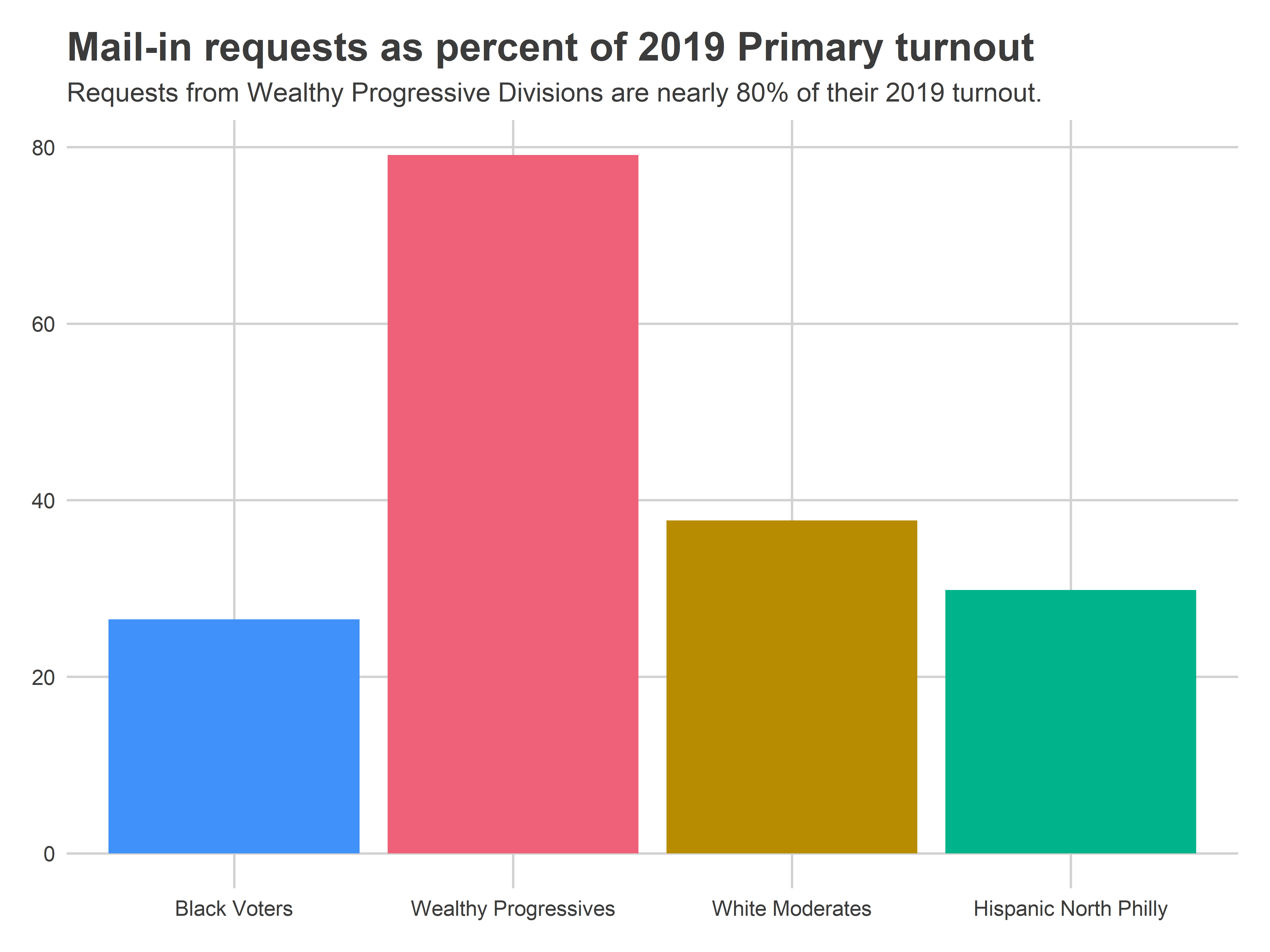
What this means for the election
Since we’ve never had mail-in voting before and it’s been over 100 years since the last pandemic, it’s impossible to know what this means for total turnout in June.
Two things are possible:
These mail-in percents represent the actual turnout. Voters decide not to vote in person, and Wealthy Progressives vastly over-represent the electorate.
Voters that aren’t requesting mail-in ballots are just planning to vote in person, and the gap totally closes on Election Day. The city-wide turnout looks normal.
Probably, the outcome will be somewhere in between. What does that mean for PA-1 and other local races? Coming soon!
Appendix: Division Maps
View code
divs %<>%
  mutate(
    popup = sprintf(
      paste(
        c(
          "<b>Division %s</b>",
          "Active registered voters: %s",
          "Mail-in requests: %s",
          "Votes in the 2019 Primary: %s",
          "Votes in the 2016 Primary: %s"
        ),
        collapse = "<br>"
      ),
      warddiv,
      scales::comma(n_reg),
      scales::comma(n_mail),
      scales::comma(round(`2019_primary`)),
      scales::comma(round(`2016_primary`))
    )
  )


divs$color_mail <- divs$n_mail
div_color_mail <- make_leaflet(
  divs,
  "color_mail",
  "Number of mail-in requests"
)
knitr::opts_chunk$set(widgetframe_self_contained = TRUE)
frameWidget(div_color_mail)
View code
divs$color_mail_vs_reg <- 100 * divs$n_mail / divs$n_reg
l0 <- make_leaflet(
  divs,
  "color_mail_vs_reg",
  "Mail-in requests as % of active registered voters",
  is_percent=TRUE
)
knitr::opts_chunk$set(widgetframe_self_contained = TRUE)
frameWidget(l0)
View code
divs$color_mail_vs_2019 <- 100 * divs$n_mail / divs$`2019_primary`
l1 <- make_leaflet(
  divs,
  "color_mail_vs_2019",
  "Mail-in requests as % of 2019 Primary voters",
  is_percent=TRUE
)
knitr::opts_chunk$set(widgetframe_self_contained = TRUE)
frameWidget(l1)
View code
divs$color_mail_vs_2016 <- 100 * divs$n_mail / divs$`2016_primary`
l2 <- make_leaflet(
  divs,
  "color_mail_vs_2016",
  "Mail-in requests as % of 2016 Primary voters",
  is_percent=TRUE
)
knitr::opts_chunk$set(widgetframe_self_contained = TRUE)
frameWidget(l2)
Any chance you can keep this uptodate every few days or so until
June 2? It will energize those of us working to get more applications completed.
Thanks
Howard
Good idea! I can try manually, whenever I get data from the office.
What is the basis upon which to dub the more wealthy Democrats as “Progressives”??
Aren’t they more likely to be Liberals (moderates)?
That’s a good question, and I spent some time debating it.
These voting blocs all come directly from which candidates did particularly well, and in this case those candidates are Gym, Brooks, and to a lesser extent Krasner. There are definitely more nuances at a finer grain, but at this crude four-bloc level, the candidates that do especially well in Center City and (especially) the ring around it actually do tend to be the progressives.