Author: Jonathan Tannen

The Live Turnout Tracker is back. And it’s got some new bells and whistles.

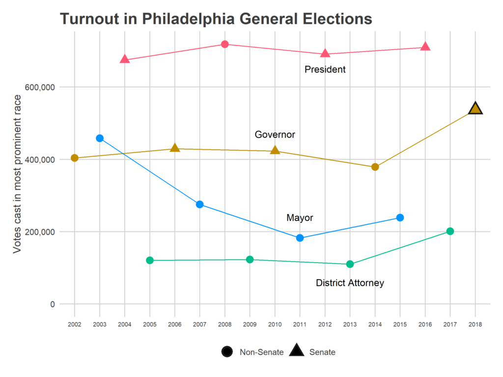
I’ve projected that Philadelphia is on pace for a record turnout year, estimating that 460,000 Philadelphians will vote on November 6th. This would beat every midterm election at least since 2002. Can we really do it? Let’s watch in real time!

What it is
The Turnout Tracker is a tool for all of us voters to share our information to generate real-time vote counts on Election Day. When you vote in Philadelphia, just record your Voter Number at your precinct (you’ll be able to see it when you sign in). Then share it here: bit.ly/sixtysixturnout

I’ll aggregate the submissions, do a little bit of math, and estimate the current number of voters across the city. You can follow it here on election day: jtannen.github.io/election_tracker.html

The Model
The model is largely the same as the primary. You can read about what it does here: announcing-the-live-election-tracker.html
​
​I’ve changed a few things, given the Primary’s post-mortem. In May, I used too much smoothing, and the result was that I missed the collapse in voting between 7-8pm due to the ill-timed thunderstorm. Worse, so many people participated that I could have gotten away with a lot less smoothing, so the error was avoidable.

This time around, I’ve built an adaptive smoother based on the number of datapoints. In connection, I’m going to bootstrap the uncertainty for every prediction, instead of using a parametric estimate. Non-parametric smoothers (the algorithm that gives me my curvy line) are particularly noisy around the edges. Unfortunately, the edge is exactly what we care about most: the final turnout is the estimate right at 8pm, the edge of our window. Making the model more responsive to short-term changes in trajectory also means it could overfit data points right at 7:59, and really mess up the curve. Bootstrapping addresses this by resampling the observed datapoints at random, giving a range of estimates that aren’t all dependent on the same points. The result is that it should correctly identify the true amount of noise right at 8pm, and give wide enough uncertainty accordingly. This will make my estimates less certain–and the plausible range larger–but hopefully allow the model to be robust to drastic end-of-day bends. And the more people that participate, the more the model will adapt to small signals, and the better result we’ll get.

What I need from you
Vote! Get your friends to vote! Then have everyone share their voter number at bit.ly/sixtysixturnout. Y’all came up huge last time around, and I’m hoping we can do it again.

See you on November 6th!

Ok, I’ve gotten a ton of great engagement, and some ideas from you all for questions to ask of the model.

In doing so, I found that it was treating a certain candidate very weirdly: incumbent candidates who were uncontested in the last race. Usually it’s bad form to change a model after you see the results, but this feels more like a bug than post-hoc analysis. So I’ve updated my model, and the results have changed fairly significantly.

What was off?

I thought I’d write up a post about what my model thought about incumbency, and pretty quickly found an issue. I rely very heavily on prior elections’ results, and when a candidate hadn’t been contested before, I was using a combination of prior Presidential results and congressional results. It turns out this was a bad idea: I was predicting that about 30% of these candidates would lose. Instead, in the last 8 elections that number has been about 5%.

How did I miss this? The model was performing well on past years, and this imbalance didn’t have any impact there. But this year, we have a fundamental change in the number of contested races, and the balance between Democrats and Republicans. In 2016, there were 43 uncontested Democrats and 50 uncontested Republicans. In 2014, there were 56 and 57.  In 2012, 45 and 49. This year, there are 55 uncontested Democrats and *23* uncontested Republicans. That huge gap multiplied this error, and gave Democrats about 5.5 too many seats.[1]

​The New Model
Since I think this is a bug, rather than a modelling decision, I decided to commit the cardinal sin of refitting the model after seeing the results. I basically changed it to treat incumbents who were uncontested the last year as a completely separate category, and the results are that (a) they do way better than I was predicting, and (b) the model is much more confident in the results. That combination of Democrats being expected to win 5.5 fewer seats, and the uncertainty shrinking, means that the probability of Dems getting over the 101.5 seat threshold is much (much) smaller.

New Predictions: 
Average Result: R 107, D 96
90% Range of Predictions:  R 115, D 88 — R 99, D 104
Probability of winning the House: R 87%, D 13%

How did seats change?
Two seats were big clues to what was going wrong with the model: 127 and 177.

Reading’s seat 127 has been represented by Thomas Caltagirone for the last 41 years. He’s facing his first challenger since 2002. And yet my model gave him essentially even odds. Why? Because his district was basically even in the 2016 US Congressional race. I was relying too heavily on the last results from other races, pretending those were state house results. The new model? Gives him an 88% chance of keeping his seat.

Seat 177 is familiar to Philadelphians as Rep. John Taylor’s former seat, being contested by Patty Kozlowski (R) and Joe Hohenstein (D). It only gave Hohenstein a 34% chance of winning despite the fact that the longtime incumbent had stepped down, and Clinton won the district handily. This one was a weirder bank shot: I wasn’t giving John Taylor his due as a candidate, so I was instead scoring the district as more Republican than it really was, and when Hohenstein lost the district in 2016, scoring him weaker than I should. The new model realizes Taylor was a strong candidate in a quite Blue district, and gives Hohenstein now a 66% chance of winning.

Overall, it is able to better differentiate candidates, and separate them from the 50% threshold. This means that there’s a lot less noise in the model, which gives Democrats less chance to surge over 101.5.

[See the seat-by-seat results here]

Ok, that’s it. Sorry for the thrash. Time to go build the Turnout Tracker.

​Sources
Data comes from the amazing Open Elections Project.
I also leaned heavily on Ballotpedia to complement and extend the data.
GIS data is from the US Census.

Footnotes
[1] These numbers don’t include cases where candidates run as e.g. D/R, which always happens in a few uncontested races (5 in 2016, 2 in 2014, 6 in 2012). For the model, I do impute their party based on other elections.