Announcing the Live Election Tracker!

Philadelphia’s 2018 Primary elections are coming on May 15th. I’m excited to announce that Sixty-Six Wards will be *live tracking* turnout on election day. And I need help from you!

What I need from you
On election day, vote! When you sign in to vote, you can see what number voter you are in your division. After voting, log in to at bit.ly/sixtysixturnout and share with me your (1) Ward, (2) Division, (3) Time of Day, and (4) Voter Number. Using that information, I’ve built a model that estimates the turnout across the city (see below).

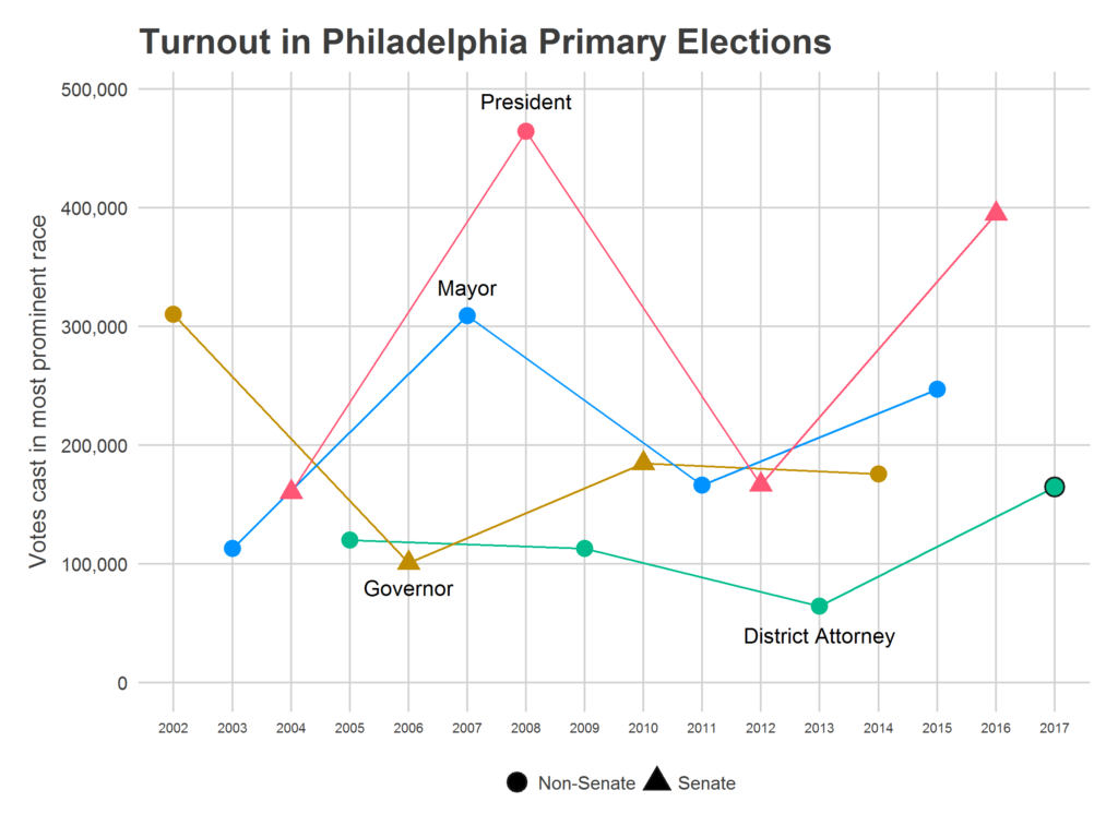
You’ll then be able to track the live election results at jtannen.github.io/election_tracker. Will turnout beat the 165,000 who voted in 2014, even with a non-competitive Senate and Governor primary? Will the surge seen in 2017 continue?

This estimation can only get better with more data points. So encourage your friends to vote, and share their voter number too!

Some note about the data collection: I only collect the four data points above (Ward, Division, Time, and Voter Number), and no identifying information on submitters. I *will* share this data publicly–again, only those four questions–in hopes that it can prove useful to others. And I am only using Democratic primary results (sorry Republicans, but there are simply too few of you, especially in off-presidential years, for me to think I could make any valid estimate).

The Model
Now for what you really care about: the math.

Estimating turnout live requires simultaneously estimating two things: each Division’s relative mobilization and the time pattern of voters throughout the day. The 100th voter means something different in a Division that had 50 voters in 2014 than it does in a Division that had 200, and it means something different at 8am than it does at 7pm. Further, Philadelphia has 1,686 Divisions, and I don’t think we’ll get data on every Division (no matter how well my dedicated readers blast out the link). I use historic correlations among Divisions to guess the current turnout in Divisions for which no one has submitted data.

To estimate turnout, I model the turnout X in division i at time t, in year y, as
log(X_ity) = a_y + b_ty + d_iy + e_ity

The variable a represents the overall turnout level in the city for this year. b_t is the time trend, which starts at exp(b_t) = 0 and finishes at exp(b_t) = 1 so the time trend progresses from 0% of voters having voted at 7am to 100% having voted at 8pm. d_i represents Division i‘s relative turnout versus other divisions for this year, and e_it is noise.

Modeling Divisions
To best estimate d_i, especially for Divisions with no submitted data, I use historical data. Using the Philadelphia primaries since 2002 (excluding 2009, where something is weird with the data), I estimate each Division’s average relative turnout versus other Divisions (its “fixed effect”), and the correlation among Divisions’ log turnout across years. Divisions are often very similar to each other: when one Division turns out strongly in an election, similar Divisions do too.

Here are the estimated average relative turnouts (the fixed effects):

We see a familiar pattern. Center City, Germantown and Mount Airy, and Overbrook all vote at disproportionately high rates, while the universities, North Philly, and the northern River Wards vote at disproportionately low rates.

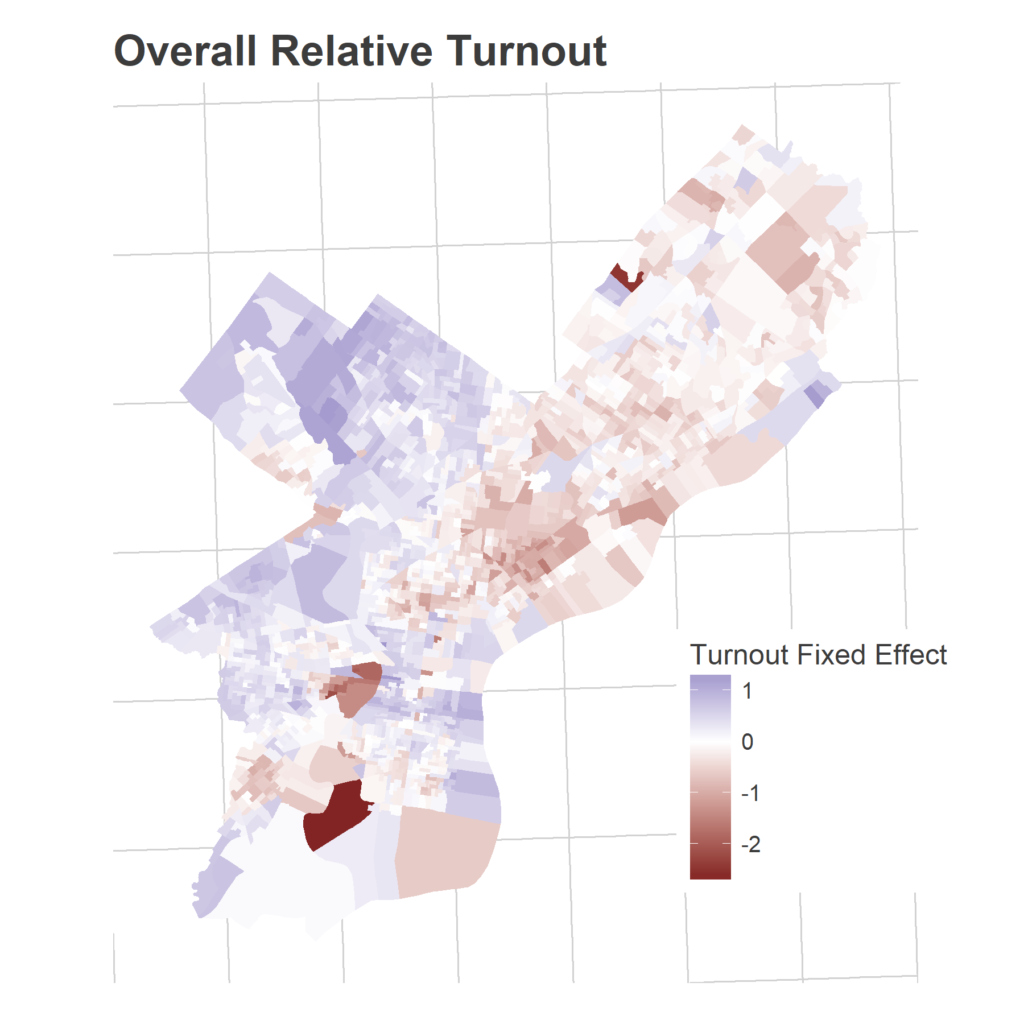
That’s across all years. But the way Divisions over- or under-perform these averages in a given year creates patterns as well. Divisions’ turnouts are correlated with each other.

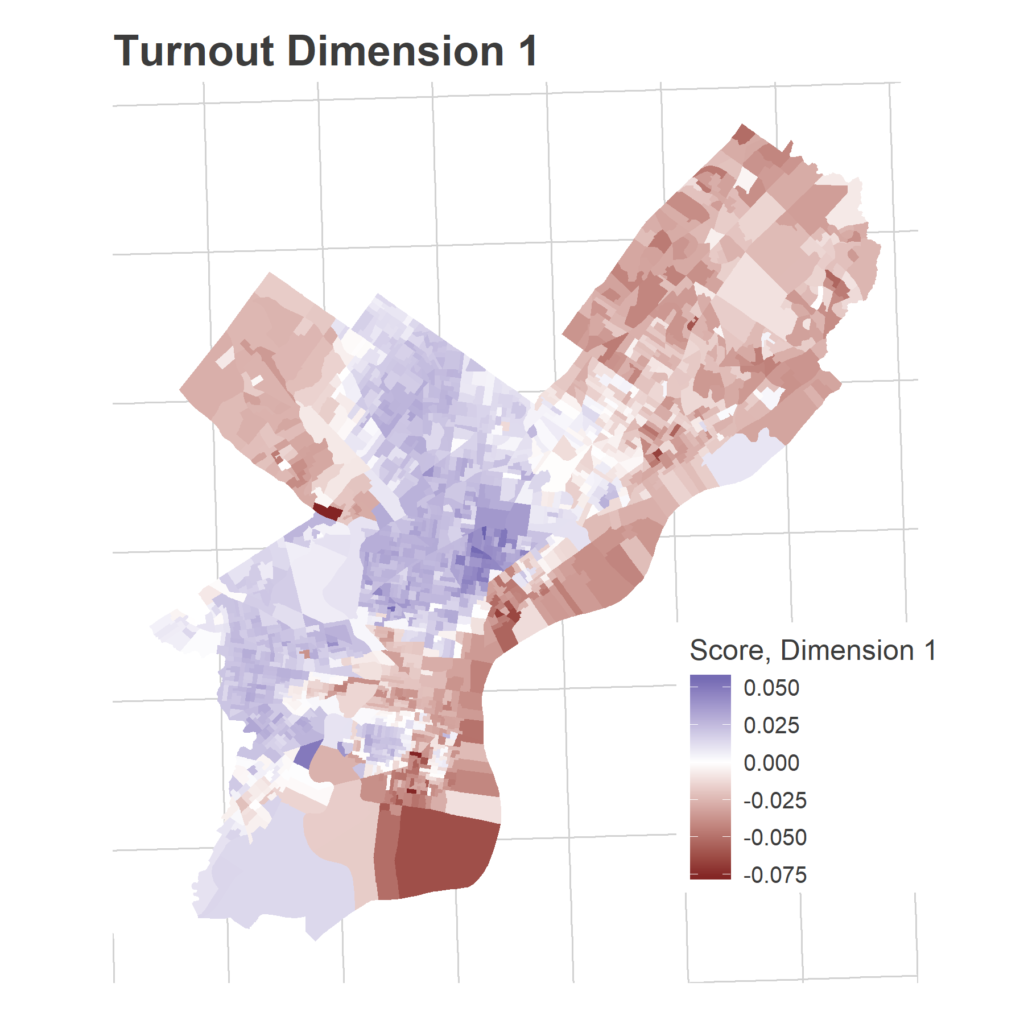
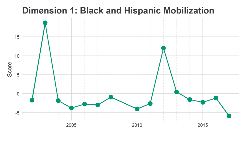
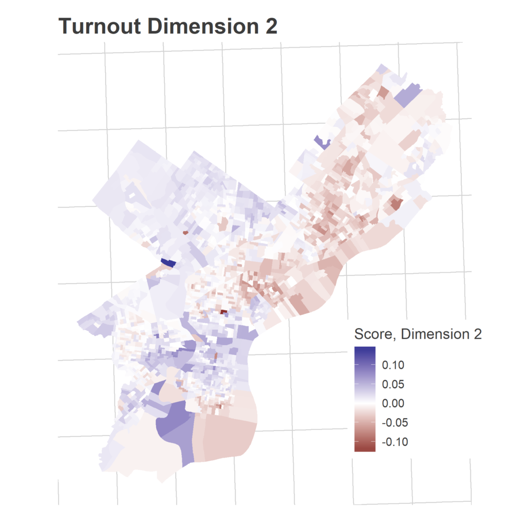
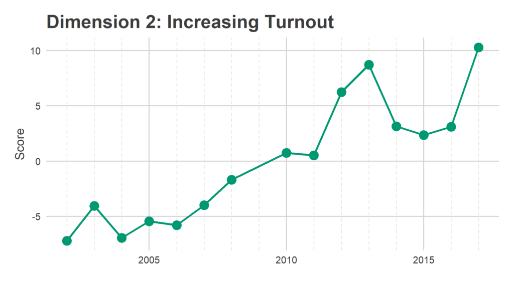
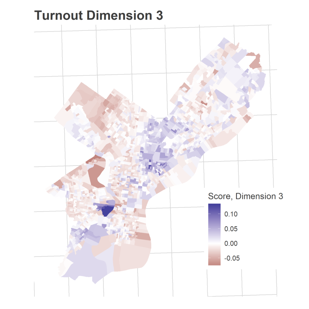
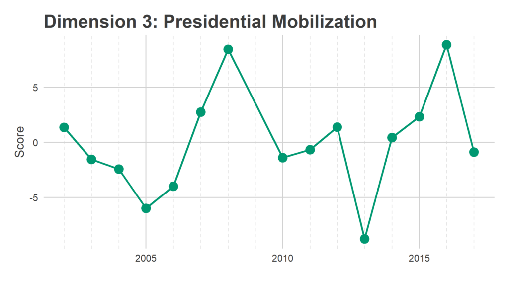
We have 1,686 Divisions and only 16 years, so we need to simplify the covariance matrix to estimate covariance among Divisions. To do that, I use Singular-Value Decomposition to identify three dimensions of turnout. These dimensions represent groups of Divisions that swing together: when one Division in the group turns out higher than usual, the others do to. The signs are not meaningful; some years the Divisions with a positive sign turn out higher, other years those with negative signs. What’s important is that the positive and negative signs move oppositely​.

SVD assigns a score in each dimension for the dimensions and for the years. Divisions with a positive score in a dimension turn out more strongly in years with positive scores, Divisions with a negative score turn out more strongly in years with negative scores.

Eyeballing the score maps together with the years’ scores serves as a sanity check for years, and provides intuition to the underlying story. The dimensions are ordered from the strongest separation to the weakest. I’m not going to pay too close attention to the specific values of the scores, what matters most is the relative values.

Dimension 1 has clearly identified the racial divide in the city. Divisions with positive scores are predominantly Black and Hispanic, while divisions with negative scores are predominantly White (again, the signs are not meaningful). Divisions with positive scores voted disproportionately in 2012 and 2003 (President Obama’s and Mayor Street’s reelections, respectively), while divisions with negative scores turned out particularly strongly in 2017.  Interestingly, the year with the lowest score, meaning the greatest disproportionate turnout in non-Hispanic White neighborhoods, was the 2017 DA’s race won by Larry Krasner.

It’s less obvious from the map what Dimension 2 captures, but the time series is clear: Dimension 2 identifies Divisions where relative turnout has steadily increased over the 16 years. This also lines up with the neighborhoods that have gentrified: Powelton, Fishtown, Fairmount, and Girard Estates have seen the strongest trends up, while broad swaths of North Philly and the Greater Northeast have seen relative decreases over time.

Dimension 3 identified Divisions that surge in turnout specifically for Presidential primaries. Penn and Drexel obviously see the strongest swings, though Southwest Philly and Hispanic sections of North Philly also have positive scores: these neighborhoods voted strongly in 2016 and 2008, relative to their typically low overall turnout.

These dimension allow me to calculate the smoothed covariance matrix Sigma, among divisions. In a given year, then, the vector of Division effects, d, is drawn from a multivariate Normal:
d ~ MVNormal(mu, Sigma),
with mu the Division fixed effects.

Time Series
The time series of voting throughout the day is currently completely unknown. What fraction of voters vote before 8am? What fraction at lunch time? Knowing how to interpret a data point at 11am hinges on the time profile of voting. For this model, I assume that all Divisions have the same time profile: all divisions have the same fraction of their voters vote before time t, with possible noise. Since I don’t have historical data for this, I will estimate it on the fly.

I model the total time effect including the annual intercept, a_y + b_t, using a loess smoother.

The full model
Having specified each term in
log(X_ity) = a_y + b_ty + d_iy + e_ity,
I fit this model using Maximum Likelihood.

The output is a joint modeling of (a) the time distribution across the city and (b) the relative strength of turnout in neighborhoods. Come election day, you’ll be able to see estimates of the current turnout, as well as how strong turnout is in your neighborhood!

See you on Election Day!
2018 could be an exciting moment for Philadelphia elections. The primary will give us an important signal for what to expect in November. Please help us generate live elections by voting, sharing your data, and getting your friends to do the same. See you May 15th!