[Guest post by Hillary Do]
What happens when you combine election season with a global pandemic? Lots and lots of mail-in ballot requests.
On May 9th, 2020 Jonathan analyzed who requested mail-in ballots. Now that the primaries are over, I wanted to take a look at what the updated data shows us.
Who’s requesting mail-in ballots and how?
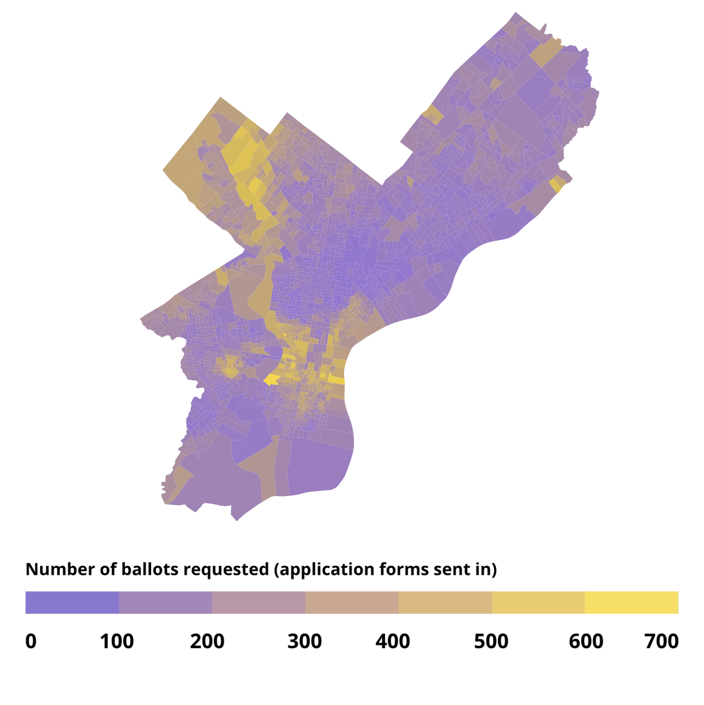
At a glance, divisions in Center City, Northwest Philly, and University City had the largest number of mail-in ballot requests. Let’s use Sixty-Six Wards’s voting blocs to take a deeper look.
These Blocs use voting patterns to categorize Divisions (so “Black Voter” divisions are not all Black Voters, but all voters from Divisions that vote disproportionately for candidates that do well in predominantly-Black Divisions).


When compared to active voters, Wealthy Progressive divisions still have the largest percent of mail-in ballot requests, despite the fact that Black voters represent nearly half of active voters. When compared to the total turnout (in person and by mail-in ballot) during the primaries this year, requests from Wealthy Progressive divisions made up 90% of their actual turnout.

These numbers matter, especially in a pandemic. Vote-by-mail is the sole way to reduce the spread of COVID-19 that may occur at polling places and we may be in the midst of our second wave in November.
Black Americans have a mortality rate from COVID-19 3.6x that of white Americans (APM Research Lab). 8 out of 10 deaths in the US have been in adults 65 years and older (CDC). Of the four voting blocs, White Moderate divisions have the highest average percentage of 65 and older residents – 24%, compared to 17%, 20%, and 14% for Wealthy Progressives, Black Voters, and Hispanic North Philly, respectively. (US Census)
Something needs to be done, but first: why is this happening? What explains the stark difference between the use of mail-in ballots in Wealthy Progressive divisions compared to the other three voting blocs? For these voting blocs, it could be that their voters:
- Didn’t know mail-in ballots were an option
- Knew that the mail-in ballots were an option, but chose not to vote-by-mail
- Distrust of the mail-in ballot system
- Preference to vote at the polls / lower coronavirus risk perception
- Too late to apply for one by the time they wanted to
- Mail-in ballot was too complicated (language barrier, number of questions, etc)
The answer is probably a mix of the above, but our city has complete control over #1 and #2C. To address #1 (Didn’t know mail-in ballots were an option), the City should mail every registered voter a mail-in ballot application form with clear, comprehensive directions on how to complete it. Why mail, you ask?

As a percent of total mail-in requests, Wealth Progressive divisions had the highest proportion of mail-in requests come online. Not every Philadelphian has access to the internet or a computer, an issue compounded by the Free Library system remaining closed.
To address #2C (Too late to apply for a mail-in ballot by the time they wanted to), the City needs to do it early, i.e. start now. What about #2A, #2B and #2D? While the City does not have complete control over these factors, they have some influence. One solution is to intensely promote voter education about mail-in ballots online, over mail, on TV, and through ward leaders. The goal would be to dispel misinformation and thoroughly explain the process to apply for one, offering multiple languages.
When are ballots being sent?
In an ideal world, after an application is received, a mail-in ballot is immediately sent. A world facing a global pandemic, however, is far from ideal. For the primaries, most ballots were sent after May 5th. 102,214 ballots, forty-five percent of the total requested, were sent after May 19th, less than the two weeks before Election Day. Of those, 27,109 could have been sent prior to May 19th. According to USPS, two weeks is not sufficient time for mail to be sent, received, sent back and then received again. One week is needed for mail to be guaranteed delivery by a certain date. Fortunately, on Election Day Eve, the Governor extended the mail-in ballot deadline to June 9th, so long as it was postmarked by June 2nd.
Of the 225,435 ballot applications, 175,176 completed ballots were eventually returned according to the City Commissioner’s final June 17th count. Somewhere along the way 50,259 ballots were not returned. There could be many reasons for this gap – missing ballots that got lost in the mail, a change in decision to vote at the polling place, or ballots that arrived past the extended June 9th deadline. One way to help close this gap is to move up the mail-in ballot timeline. Mail everyone a mail-in ballot application form now so any of those reasons can be addressed within a reasonable time frame. Voters can make plans to track down a missing ballot and feel confident their ballot will arrive in time.
In doing this analysis, I also want to acknowledge what the data doesn’t show. It doesn’t show the amount of work that goes behind an election during a global pandemic. It doesn’t show the tedious work of processing tens of thousands of ballots. It doesn’t show the sudden onslaught of unexpected factors that now change how people can vote safely.
However, now that we’ve been through the first round of elections in a COVID-19 world, it’s our City’s duty to sufficiently prepare for the next one. What the data shows is a stark difference in mail-in ballot requests among various city pockets, with a higher request rate in Wealthy Progressive divisions. Many factors could be creating this result, including demographics like race, age, and subsequently, computer access, confidence in a mail-in ballot system, a strong neighborhood polling place culture, and more.
Moreover, the data reveals that time is of the essence and advises us as to what we can do going forward. We have until November to prepare. We have (more) time and information, as well as a city of resilient, caring people who will offer their help to protect our elections. The City needs to make a plan, starting now. Philly voters deserve an election that ensures safe, equal, and guaranteed access to the ballot box.