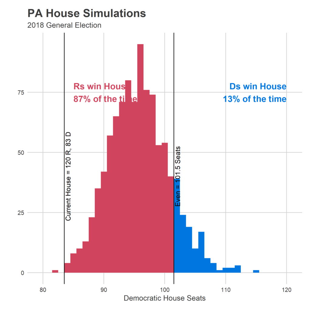
In doing so, I found that it was treating a certain candidate very weirdly: incumbent candidates who were uncontested in the last race. Usually it’s bad form to change a model after you see the results, but this feels more like a bug than post-hoc analysis. So I’ve updated my model, and the results have changed fairly significantly.
What was off?
This is neat stuff, but I suspect it isn’t giving enough weight to the power of incumbency [which is a nerdy way of saying that I think the GOP will keep control of the house[ https://t.co/pkFo9zTAMp
— Jim Saksa (@saksappeal) October 24, 2018
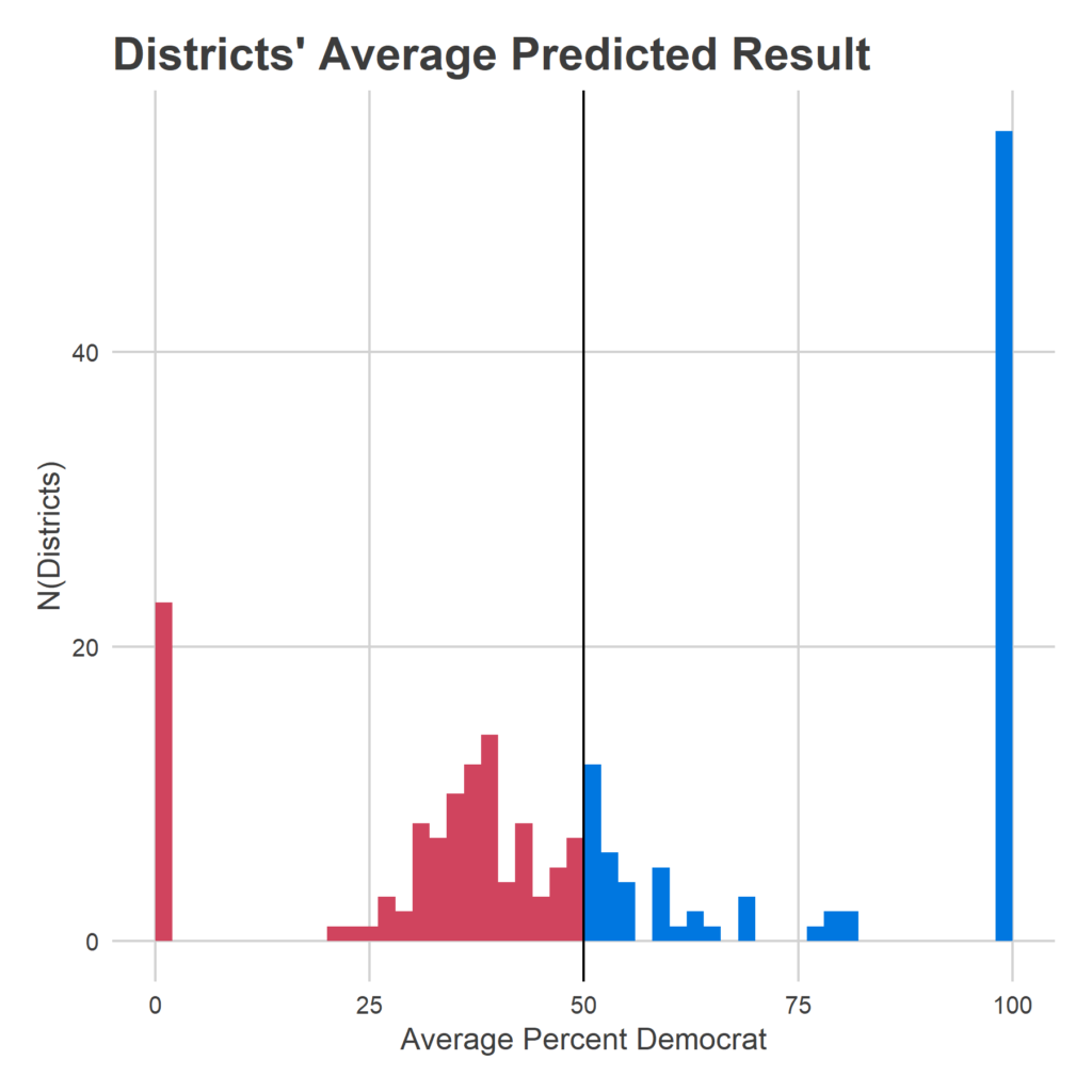
How did I miss this? The model was performing well on past years, and this imbalance didn’t have any impact there. But this year, we have a fundamental change in the number of contested races, and the balance between Democrats and Republicans. In 2016, there were 43 uncontested Democrats and 50 uncontested Republicans. In 2014, there were 56 and 57. In 2012, 45 and 49. This year, there are 55 uncontested Democrats and *23* uncontested Republicans. That huge gap multiplied this error, and gave Democrats about 5.5 too many seats.[1]
The New Model
Since I think this is a bug, rather than a modelling decision, I decided to commit the cardinal sin of refitting the model after seeing the results. I basically changed it to treat incumbents who were uncontested the last year as a completely separate category, and the results are that (a) they do way better than I was predicting, and (b) the model is much more confident in the results. That combination of Democrats being expected to win 5.5 fewer seats, and the uncertainty shrinking, means that the probability of Dems getting over the 101.5 seat threshold is much (much) smaller.
New Predictions:
Average Result: R 107, D 96
90% Range of Predictions: R 115, D 88 — R 99, D 104
Probability of winning the House: R 87%, D 13%

Two seats were big clues to what was going wrong with the model: 127 and 177.
Reading’s seat 127 has been represented by Thomas Caltagirone for the last 41 years. He’s facing his first challenger since 2002. And yet my model gave him essentially even odds. Why? Because his district was basically even in the 2016 US Congressional race. I was relying too heavily on the last results from other races, pretending those were state house results. The new model? Gives him an 88% chance of keeping his seat.
Seat 177 is familiar to Philadelphians as Rep. John Taylor’s former seat, being contested by Patty Kozlowski (R) and Joe Hohenstein (D). It only gave Hohenstein a 34% chance of winning despite the fact that the longtime incumbent had stepped down, and Clinton won the district handily. This one was a weirder bank shot: I wasn’t giving John Taylor his due as a candidate, so I was instead scoring the district as more Republican than it really was, and when Hohenstein lost the district in 2016, scoring him weaker than I should. The new model realizes Taylor was a strong candidate in a quite Blue district, and gives Hohenstein now a 66% chance of winning.
Overall, it is able to better differentiate candidates, and separate them from the 50% threshold. This means that there’s a lot less noise in the model, which gives Democrats less chance to surge over 101.5.

Ok, that’s it. Sorry for the thrash. Time to go build the Turnout Tracker.
Sources
Data comes from the amazing Open Elections Project.
I also leaned heavily on Ballotpedia to complement and extend the data.
GIS data is from the US Census.
Footnotes
[1] These numbers don’t include cases where candidates run as e.g. D/R, which always happens in a few uncontested races (5 in 2016, 2 in 2014, 6 in 2012). For the model, I do impute their party based on other elections.