With a tense race for District Attorney and the typically-packed race for Common Pleas, we’re all looking for any signals we can get.
The friendly folks at the Commissioners’ Office have shared mail-in ballot requests with me, so let’s dig in.
View code
library(dplyr)
library(tidyr)
library(ggplot2)
library(sf)
library(scales)
devtools::load_all("../../admin_scripts/sixtysix/")
mail <- readxl::read_xlsx(
"../../data/raw_election_data/Vote by Mail Listing (5-11-21).xlsx",
sheet = "Voter Listing"
)
dup_ids <- mail$`ID Number`[duplicated(mail$`ID Number`)] %>% unique()
mail_dup <- mail %>% filter(`ID Number` %in% dup_ids)
mail <- mail %>% filter(!`ID Number` %in% dup_ids)
mail_dup <- mail_dup %>%
group_by(`ID Number`) %>%
summarise(
across(
c(AppReturnedDate, BallotSent, BallotReturned),
function(var){
if(all(is.na(var))) return(NA)
max(var, na.rm=T)
}
),
PartyDesc=ifelse(any(PartyDesc=="DEMOCRATIC"), "DEMOCRATIC", PartyDesc[1])
)
mail <- bind_rows(mail, mail_dup)
df_major <- readRDS("../../data/processed_data/df_major_type_20210118.Rds")
head(df_major)
n_mail <- mail %>%
filter(PartyDesc=="DEMOCRATIC") %>%
mutate(ret = !is.na(BallotReturned)) %>%
group_by(ret) %>%
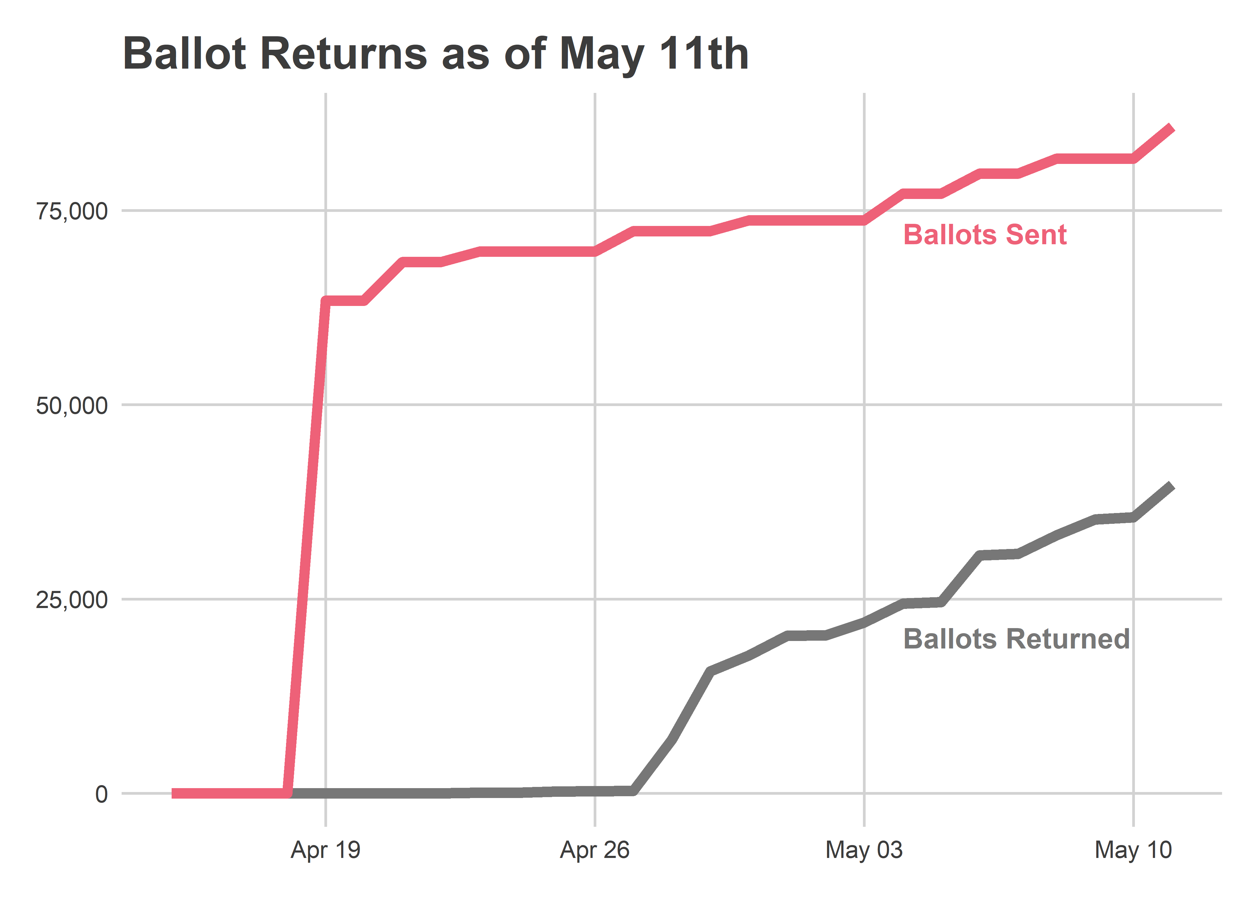
count()Some 78,178 Democratic voters requested ballots, and 35,802 of them had already been returned as of May 11th. That suggests we’ll get close to the 155,000 votes cast in 2017.
View code
turnout <- df_major %>%
  filter(is_topline_office) %>%
  filter(election_type=="primary", party=="DEMOCRATIC") %>%
  group_by(year, ward, type) %>%
  summarise(votes=sum(votes)) %>%
  group_by(year, ward) %>%
  mutate(total=sum(votes)) %>%
  ungroup() %>%
  pivot_wider(names_from="type", values_from="votes", values_fill = list(votes=0))

cycle <- function(year){
  year <- asnum(year)
  cycle_num <- year %% 4
  c("President", "District Attorney", "Governor", "Mayor")[cycle_num+1]
}

ggplot(
  turnout %>% group_by(year) %>%
    summarise(across(A:total, sum)) %>%
    mutate(
      cycle=cycle(year)
    ),
  aes(x=asnum(year), y=total, color=cycle)
) +
  geom_line(aes(group=cycle), size=2) +
  scale_color_manual(
    values=with(
      colors_sixtysix(),
      c(
        President = light_red, `District Attorney`=light_green,
        Governor = light_orange, Mayor = light_blue,
        "2021 Mail-In\nRequests"=light_green
      )
    ),
    guide=FALSE
  ) +
  theme_sixtysix() +
  expand_limits(y=0) +
  scale_y_continuous(labels=scales::comma) +
  geom_point(
    data=data.frame(year=2021, total=sum(n_mail$n), cycle="District Attorney"),
    size=4
  ) +
  geom_text(
    data=tribble(
      ~year, ~cycle, ~total,
      2016, "President", 370e3,
      2015.5, "Mayor", 250e3,
      2015.2, "Governor", 190e3,
      2012, "District Attorney", 40e3,
      2018.7, "2021 Mail-In\nRequests", 40e3
    ),
    hjust=0,
    size=4,
    aes(label=cycle)
  )+
  labs(
    title="Votes in Democratic Primaries",
    y="Votes cast for topline office",
    x=NULL,
    fill=NULL
  )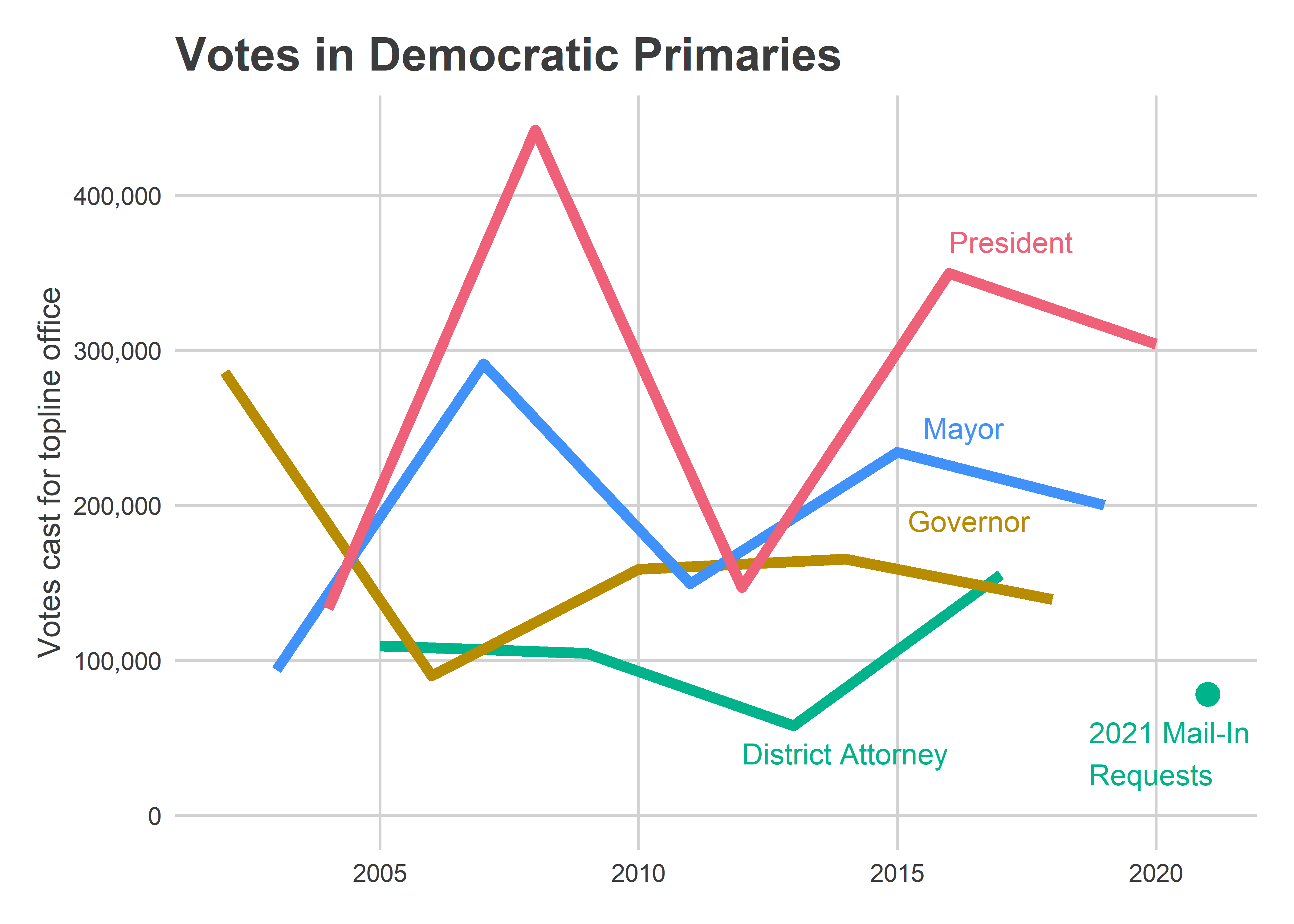
But there are big unknowns in what mail-in requests tell us about overall turnout. We’ve only had two elections with no-excuse mail-in voting, and this might be the first where we’ll see close to “normal” mail-in use. For last year’s elections, we were both at the height of the pandemic and we saw mail-ins became politically polarized. In this election I expect mail-in usage to be much more a function of convenience to individual voters. That would mean ward counts will be closer to proportional to overall turnout, but will still deviate in ways that we don’t today know; there’s no past data.
View code
library(leaflet)

make_leaflet <- function(
  df,
  title=NULL,
  fill_col="fill",
  popup_col="popup",
  zoom=11
){

  pal <- cut_vals(df[[fill_col]])

  legend <- create_legend(
    pal$min,
    pal$max,
    pal$step_size,
    pal$pal
  )

  init_map(df, zoom) %>%
    addPolygons(
      data=df$geometry,
      weight=0,
      color="white",
      opacity=1,
      fillOpacity = 0.8,
      smoothFactor = 0,
      fillColor = pal$pal(df[[fill_col]]),
      popup=df[[popup_col]]
    ) %>%
    addControl(title, position="topright", layerId="map_title")  %>%
    addLegend(
      layerId="geom_legend",
      position="bottomright",
      colors=legend$colors,
      labels=legend$labels
    )
}

init_map <- function(data, zoom){
  bbox <- st_bbox(data)

  leaflet(
    options=leafletOptions(
      minZoom=zoom,
      maxZoom=zoom,
      zoomControl=TRUE,
      dragging=FALSE
      )
  )%>%
    setView(
      zoom=zoom,
      lng=mean(bbox[c(1,3)]),
      lat=mean(bbox[c(2,4)])
    ) %>%
    addProviderTiles(providers$Stamen.TonerLite) %>%
    setMaxBounds(
      lng1=bbox["xmin"],
      lng2=bbox["xmax"],
      lat1=bbox["ymin"],
      lat2=bbox["ymax"]
    )
}

cut_vals <- function(x){
  min_value <- min(x, na.rm=TRUE)
  max_value <- max(x, na.rm=TRUE)

  sigfig <- round(log10(max_value-min_value)) - 1
  n_steps <- (max_value-min_value)/10^sigfig
  step_size <- ifelse(n_steps >= 10, 2, 1) * 10^(sigfig)

  min_value <- step_size * floor(min_value / step_size)
  max_value <- step_size * ceiling(max_value / step_size)

  pal <- colorNumeric(
    "viridis",
    domain=c(min_value, max_value)
  )

  list(
    min=min_value,
    max=max_value,
    step_size=step_size,
    pal=pal
  )
}

create_legend <- function(
  min_value,
  max_value,
  step_size,
  pal
){
  legend_values <- seq(min_value, max_value, step_size)
  legend_colors <- pal(legend_values)
  legend_labels <- scales::comma(legend_values,accuracy=step_size)

  list(
    colors=legend_colors,
    values=legend_values,
    labels=legend_labels
  )
}
View code
divs <- st_read("../../data/gis/warddivs/202011/Political_Divisions.shp", quiet=T) %>%
  mutate(warddiv = sprintf("%s-%s", substr(DIVISION_N,1,2), substr(DIVISION_N, 3, 4)))

wards <- st_read("../../data/gis/warddivs/201911/Political_Wards.shp", quiet=T) %>%
  mutate(ward = sprintf("%02d", asnum(WARD_NUM)))

mail_div <- mail %>%
  filter(PartyDesc=="DEMOCRATIC") %>%
  mutate(warddiv = paste0(Ward, "-", Division)) %>%
  group_by(warddiv) %>%
  summarise(
    apps = sum(!is.na(AppReturnedDate)),
    ballots = sum(!is.na(BallotSent)),
    returned = sum(!is.na(BallotReturned))
  )

mail_ward <- mail_div %>%
  mutate(ward = substr(warddiv, 1, 2)) %>%
  group_by(ward) %>%
  summarise(across(apps:returned, sum))

turnout_2020_gen <- df_major %>%
  filter(year==2020, election_type=="general", is_topline_office) %>%
  group_by(ward, type) %>%
  summarise(votes=sum(votes)) %>%
  group_by(ward) %>%
  mutate(total=sum(votes)) %>%
  ungroup() %>%
  pivot_wider(names_from=type, values_from=votes)

wards_lf <- wards %>%
  left_join(mail_ward) %>%
  left_join(turnout %>% filter(year==2017)) %>%
  left_join(turnout_2020_gen, by="ward", suffix=c("", ".20")) %>%
  mutate(
    popup=sprintf(
      paste(
        c(
          "<b>Ward %s</b>",
          "Mail-In Requests (Dem): %s",
          "Mail-In Returns (Dem): %s",
          "Votes 2017 (Dem): %s",
          "Mail-In Votes Nov 2020: %s"
        ),
        collapse = "<br>"
      ),
      ward,
      comma(apps),
      comma(returned),
      comma(total),
      comma(M.20)
    )
  )

mail_lf <- make_leaflet(wards_lf, title="Mail-In Requests", fill_col="apps")
Mail-in applications are about 30% of what we saw in November, with North Philly and the Universities significantly lagging (which is typical for turnout in Municipal versus Presidential elections).
View code
prop_lf <- wards_lf %>%
  mutate(fill=apps / M.20) %>%
  make_leaflet(title="Mail-In Requests, May 2021 / Nov 2020")
View code
library(lubridate)
mail_time <- mail %>%
  mutate(
    app = mdy(BallotSent),
    ret = mdy(BallotReturned)
  ) %>%
  select(app, ret) %>%
  pivot_longer(cols=c(app,ret), values_to = "date") %>%
  filter(!is.na(date)) %>%
  group_by(name, date) %>%
  count()

dates <- seq(from=min(mail_time$date), to=max(mail_time$date), by="days")

mail_time <- as.data.frame(expand_grid(date=dates, name=c("app", "ret"))) %>%
  left_join(mail_time) %>%
  group_by(name) %>%
  arrange(date) %>%
  mutate(n = ifelse(is.na(n), 0, n)) %>%
  mutate(cum = cumsum(n))


ggplot(
  mail_time %>% mutate(var=c(app="Ballots Sent", ret="Ballots Returned")[name]),
  aes(x=date, y=cum, color=var)
) +
  geom_line(aes(group=var), size=2) +
  theme_sixtysix() +
  scale_x_date(limits=c(ymd("2021-04-15"), max(mail_time$date))) +
  scale_y_continuous(labels=scales::comma) +
  scale_color_manual(
    values=c(
      `Ballots Sent`=colors_sixtysix()$light_red,
      `Ballots Returned`=colors_sixtysix()$strong_grey
    ),
    guide=FALSE
  ) +
  labs(
    y=NULL,
    x=NULL,
    title="Ballot Returns as of May 11th"
  ) +
  annotate(
    "text",
    x=ymd("2021-05-04"),
    y=c(20e3, 72e3),
    label=c("Ballots Returned", "Ballots Sent"),
    hjust=0,
    size=4,
    fontface="bold",
    color=colors_sixtysix()[c("strong_grey", "light_red")]
  )
Party Switches
In my post on party changes, I assumed the changes were strategic: Republicans switching to Democrats so they could vote in the closed Primary. But maybe those were just Republicans who were finally fed up with the party after January 6th?
Comparing Philadelphia to other counties provides strong evidence that the switches are, in fact, strategic. If the changes were due to distaste with the party, we might expect Philadelphia’s party switches to look like other counties. And in fact the rate of Republicans switching to a third party or independent looks the same in Philadelphia as the rest of the state. But the rate of Republicans switching to Democrats is more than five times as high in Philadelphia as any other county, including the Philadelphia suburbs and Allegheny.

View code
fve_names <- read.csv("../../data/voter_registration/col_names.csv")

read_fve <- function(ds, county="PHILADELPHIA"){
  path <- sprintf(
    "../../data/voter_registration/%1$s/%2$s FVE %1$s.txt",
    ds, toupper(county)
  )
  fve <- readr::read_tsv(
    path,
    col_types = paste0(rep("c", nrow(fve_names)), collapse=""),
    col_names = as.character(fve_names$ï..name)
  ) %>%
    mutate(
      party = case_when(
        `Party Code` %in% c("D", "R", NA) ~ as.character(`Party Code`),
        TRUE~"Oth"
      ),
    )
  fve
}

lagged_fve <- function(first, second, county="PHILADELPHIA"){
  first <- read_fve(first, county)
  second <- read_fve(second, county)
  second <- second %>%
    left_join(
      first %>% select(`ID Number`, party, `Street Name`),
      by="ID Number",
      suffix=c(".1", ".0")
    ) %>%
    mutate(
      party_switch = paste0(party.0, "_", party.1),
      ward =  substr(`Precinct Code`, 1, 2),
      warddiv = paste0(ward, "-", substr(`Precinct Code`, 3, 4)),
      county=county
    )
  second
}

if(FALSE){
  fve_21 <- lagged_fve("20201019", "20210510")
  saveRDS(fve_21, "fve_21.RDS")
} else {
  fve_21 <- readRDS("fve_21.RDS")
}

# fve_21 %>%
#   filter(!is.na(`Election 3 Vote Method`)) %>%
#   filter(party_switch %in% c("D_D", "R_D")) %>%
#   left_join(mail, by="ID Number") %>%
#   mutate(app=!is.na(AppReturnedDate), ret=!is.na(BallotReturned)) %>%
#   group_by(party_switch, app, ret) %>%
#   count()
#
# fve_21 %>%
#   filter(party_switch %in% c("D_D", "R_D")) %>%
#   left_join(mail, by="ID Number") %>%
#   mutate(app=!is.na(AppReturnedDate), ret=!is.na(BallotReturned)) %>%
#   group_by(party_switch, app, ret) %>%
#   count()
How about mail-in application rates among them? Of the 6,384 Republican to Democrat switchers, 672 have requested a mail-in ballot and 300 have returned it. That rate is higher than among Democrat registrants who stayed Democrats (77K requests out of 784K voters), but it’s lower than among the subset of those stably-Democrat registrants who also voted in November 2020 (75K requests out of 567K voters). So these party-switchers are not particularly likely to request mail-in ballots. But they also may just be planning to vote in person.