The 2021 race for Common Pleas

Sorry for the radio silence. With the 2021 Democratic Primary on May 18th, and mail-in ballots being sent out this week, it’s now or never to think out loud about this election.

I have a lot of weakly-related threads of thoughts going into this election, so I’m going to structure this post as a series of sections, each of which should probably be their own posts. Here’s what I’m looking at with a month to go in the races.

Ballot Position Winners and Losers

The Common Pleas candidates had their ballot draw, and Caroline Turner won the top spot. That first position has won in every election since at least 2009. Just being in the first column nearly triples a candidate’s votes.

2021 Sample Ballot for Common Pleas, from philadelphiavotes.com.

This year, we have a small race: sixteen candidates are contesting eight seats. Sadly, the winners are easy to predict just from structural factors; voters pay little attention to the race, so it’s hard for candidates to break through, and structural factors like ballot position dominate. In 2019, I predicted the races pretty well using just ballot position, gender, Democratic City Committee endorsements, and Philadelphia Bar Association recommendations.

Speaking of those recommendations, we have an interesting test of them this year. Two years ago was the first time the Bar’s “Highly Recommended” rating seemed to have real teeth, with three of the four candidates winning, including Tiffany Palmer with a terrible position and no DCC backing. That was the one way the simulations really failed. This year, those ratings include five Highly Recommended candidates, seven Recommended, and four Not Recommended. Four of those Highly Recommended candidates are in the second or third column, and will be trying to replicate Kyriakakis’ and Palmer’s 2019 Highly Recommended wins from poor positions.

Some other interesting things to watch:

  • This is the first year that the DCC has endorsed a slate of entirely Bar-Recommended judges, including three Highly Recommended. So that severly dampens the chances of a Not Recommended judge.
  • Five of the six first-column candidates are Recommended by the Bar, and four of those are additionally endorsed by the DCC. The only Recommended-but-not-DCC-endorsed candidate is Caroline Turner, who’s in the top ballot position, and the lone first-column candidate who was Not Recommended is second-position Terri Booker.

When I rerun my simulation model from 2019, here are the results.

View code
library(tidyr)
library(dplyr)
library(ggplot2)
library(magrittr)
library(sf)

devtools::load_all("../../admin_scripts/sixtysix")

ballot <- read.csv("../../data/common_pleas/judicial_ballot_position.csv")
ballot$name <- tolower(ballot$name)
ballot$name <- gsub("[[:punct:]]", " ", ballot$name)
ballot$name <- trimws(ballot$name)
ballot$year <- as.character(ballot$year)

df_major <- readRDS("../../data/processed_data/df_major_20210118.Rds")
df <- df_major %>%
  filter(
    office == "JUDGE OF THE COURT OF COMMON PLEAS",
    year >= 2009,
    election_type=="primary",
    party=="DEMOCRATIC"
  ) %>% 
  mutate(candidate = tolower(candidate)) %>%
  group_by(warddiv, year, candidate) %>% 
  summarise(votes = sum(votes))

df_total <- df %>% 
  group_by(year, candidate) %>% 
  summarise(votes = sum(votes))

election <- data.frame(
  year = c(2009, 2011, 2013, 2015, 2017, 2019),
  votefor = c(7, 10, 6, 12, 9, 6)
) %>% mutate(year=as.character(year))

election <- election %>% left_join(
  ballot %>% group_by(year) %>% summarise(
    nrows = max(rownumber),
    ncols = max(colnumber), 
    ncand = n(),
    n_philacomm = sum(philacommrec >= 1),
    n_inq = sum(inq),
    n_dcc = sum(dcc)
  )
)

df_total <- df_total %>% 
  inner_join(
    ballot,
    by = c("candidate" = "name", "year" = "year")
  )

df_total <- df_total %>%
  filter(candidate != "write in") 

df_total <- df_total %>%
  left_join(election, by="year") %>%
  group_by(year) %>%
  mutate(
    pvote = votes / sum(votes),
    rank=rank(desc(votes)),
    winner = rank <= votefor
  ) 

library(forcats)

prep_df_for_lm <- function(df, use_candidate=TRUE){
  df <- df %>% mutate(
    rownumber = fct_relevel(factor(as.character(rownumber)), "3"),
    colnumber = fct_relevel(factor(as.character(colnumber)), "3"),
    col1 = colnumber == 1,
    col2 = colnumber == 2,
    col3 = colnumber == 3,
    row1 = rownumber == 1,
    row2 = rownumber == 2,
    is_rec = philacommrec > 0,
    is_highly_rec = philacommrec==2,
    inq=inq>0
  )
  if(use_candidate)
    df <- df %>% mutate(
      candidate_year = paste(candidate, year, sep="::")
    )
  return(df)
}

df_complemented <- df %>% 
  mutate(ward = substr(warddiv, 1, 2)) %>%
  group_by(ward, year, candidate) %>%
  summarise(votes=sum(votes)) %>%
  group_by(ward) %>%
  mutate(pvote = votes / sum(votes)) %>%
  inner_join(
    df_total %>% prep_df_for_lm(),
    by = c("year", "candidate"),
    suffix = c("", ".total")
  ) 

library(lme4)

## better opt: https://github.com/lme4/lme4/issues/98
library(nloptr)
defaultControl <- list(
  algorithm="NLOPT_LN_BOBYQA",xtol_rel=1e-6,maxeval=1e5
)
nloptwrap2 <- function(fn,par,lower,upper,control=list(),...) {
    for (n in names(defaultControl)) 
      if (is.null(control[[n]])) control[[n]] <- defaultControl[[n]]
    res <- nloptr(x0=par,eval_f=fn,lb=lower,ub=upper,opts=control,...)
    with(res,list(par=solution,
                  fval=objective,
                  feval=iterations,
                  conv=if (status>0) 0 else status,
                  message=message))
}

if(FALSE){
  rfit <- lmer(
    log(pvote + 0.001) ~ 
      (1 | candidate_year)+
        row1 + row2 +
        I(gender == "F") +
        col1 + col2 + I(col1 * row1) +
        dcc + inq +
        is_rec + is_highly_rec +
        factor(year) +
        (
            I(gender == "F") +
            col1 + col2 + I(col1 * row1) +
            dcc + inq +
            is_rec + is_highly_rec 
          | ward
        ),
          df_complemented
  )
  saveRDS(rfit, file="rfit.RDS")
} else {
  rfit <- readRDS("rfit.RDS")
}
  
ranef <- as.data.frame(ranef(rfit)$ward) %>% 
  tibble::rownames_to_column("ward")  %>%
  gather("variable", "random_effect", -ward) %>%
  mutate(
    fixed_effect = fixef(rfit)[variable],
    effect = random_effect + fixed_effect
  )

wards <- st_read("../../data/gis/warddivs/201911/Political_Wards.shp", quiet=TRUE)
wards <- wards %>% 
  mutate(ward = sprintf("%02d", asnum(WARD_NUM))) 
ward_effects <- wards %>%  
  left_join(
    ranef,
    by=c("ward")
  )

format_effect <- function(x){
  paste0("x", round(exp(x), 1))
}

fill_min <- ward_effects %>%
  filter(
    variable %in% c(
      "col1TRUE", "col2TRUE", "dcc", "inq", "is_recTRUE", "is_highly_recTRUE"
    )
  )  %>%
  with(c(min(effect), max(effect)))

format_variables <- c(
  is_recTRUE="Recommended",
  is_highly_recTRUE="Highly Recommended",
  dcc = "Dem. City Committee Endorsement",
  inqTRUE = "Inquirer",
  col1TRUE = "First Column",
  col2TRUE = "Second Column"
)

ward_effects$variable_name <- factor(
  format_variables[ward_effects$variable],
  levels = format_variables
)

replace_na <- function(x, r=0) ifelse(is.na(x), r, x)

df_2021 <- ballot %>% 
  filter(year == 2021) %>%
  mutate(
    philacommrec = replace_na(philacommrec),
    dcc = replace_na(dcc),
    inq = (philacommrec > 0),
    year = "2019"  ## fake year to trick lm
  ) %>%
  prep_df_for_lm(use_candidate = FALSE) %>%
  left_join(
    expand.grid(
      name = unique(ballot$name),
      ward = unique(ward_effects$ward)
    )
  ) 

## pretend it's one candidate, but then marginalize over candidates
df_2021$log_pvote <- predict(
  rfit,
  newdata = df_2021 %>% 
    mutate(candidate_year = df_complemented$candidate_year[1])
)

df_2021 <- df_2021 %>%
  mutate(pvote_prop = exp(log_pvote))

sd_cand <- sd(ranef(rfit)$candidate_year$`(Intercept)`)
simdf <- expand.grid(
  sim = 1:1000,
  name = unique(df_2021$name)
) %>%
  mutate(cand_re = rnorm(n(), sd = sd_cand))

## https://econsultsolutions.com/simulating-the-court-of-common-pleas-election/
votes_per_voter <- 4.5

ward_votes <- df %>%
  filter(year == 2019) %>%
  mutate(ward=substr(warddiv, 1, 2)) %>%
  group_by(ward) %>% 
  summarise(turnout=sum(votes))

simdf <- df_2021 %>%
  left_join(simdf, by=c("name")) %>%
  mutate(pvote_prop_sim = pvote_prop * exp(cand_re)) %>%
  group_by(ward, sim) %>%
  mutate(pvote = pvote_prop_sim / sum(pvote_prop_sim)) %>%
  group_by() %>%
  left_join(ward_votes, by="ward") %>%
  mutate(votes = turnout * votes_per_voter * pvote) %>%
  group_by(sim, name) %>%
  summarise(votes = sum(votes)) 


simdf <- simdf %>%
  group_by(sim) %>%
  mutate(
    vote_rank = rank(desc(votes)),
    pvote=100*votes/sum(votes),
    winner = vote_rank <= 8
  )

remove_na <- function(x, r=0) return(ifelse(is.na(x), r, x))
View code
ggdata <-   simdf %>% group_by(sim)  %>%
    left_join(ballot %>% filter(year==2021)) %>%
    mutate(name=format_name(name)) %>%
    group_by(name, dcc, philacommrec) %>%
    summarise(
      mean = mean(pvote),
      p975 = quantile(pvote, 0.975),
      p025 = quantile(pvote, 0.025),
      .groups = "drop"
    ) %>%
    arrange(desc(mean)) %>%
    mutate(name = factor(name, levels=name))

labx <- 9.5

ggplot(
  ggdata,
  aes(x=name, y=mean)
) +
  geom_hline(
    aes(yintercept=simdf %>% filter(vote_rank==8) %>% with(mean(pvote)))
  )+
  geom_errorbar(aes(ymin=p025, ymax=p975), width=0) + 
  geom_point(
    data=ggdata %>% filter(philacommrec ==2),
    size=6,
    color="black"
  ) +
  geom_point(
    data=ggdata %>% filter(philacommrec ==1),
    size=6,
    color="grey30"
  ) +
  geom_point(
    aes(color=(dcc>0), size=as.character(philacommrec)),
    size=4
  ) +
  scale_color_manual(
    values=c(`TRUE` = colors_sixtysix()$strong_blue, `FALSE`="grey50"),
    guide=FALSE
  ) +
  scale_size_manual(
    values=c(`0` = 2, `1`=3, `2`=4),
    guide=FALSE
  ) +
  expand_limits(y=0)+
  labs(
    x=NULL,
    y="Percentage of Vote",
    title="Results over 1,000 Simulations"
  ) +
  theme_sixtysix()%+replace%
  theme(axis.text.x = element_text(angle=-90, hjust=0)) +
  annotate("text", x=11.5, y=7, hjust=0, label="Average Vote for 8th Place") +
  annotate("point", x=labx, y=17, size=4, color=colors_sixtysix()$strong_blue) +
  annotate("text", x=labx+0.4, y=17, hjust=0, label="Democratic City Committee") +
  annotate("point", x=labx, y=15, size=6, color="grey30") +
  annotate("point", x=labx, y=15, size=4, color="grey50") +
  annotate("text", x=labx+0.4, y=15, hjust=0, label="Bar Recommended")+ 
  annotate("point", x=labx, y=13, size=6, color="black") +
  annotate("point", x=labx, y=13, size=4, color="grey50") +
  annotate("text", x=labx+0.4, y=13, hjust=0, label="Bar Highly Recommended") +
  annotate("errorbar", x=labx, ymin=10.5, ymax=11.5, width=0)+
  annotate("text", x=labx+0.4, y=11, hjust=0, label="95% of simulations")

Remember, this model did pretty well in 2019, with the huge exception of underestimating the value the Bar’s High Recommendation. Four of the Highly Recommended candidates are hanging around 50% chances of winning–Hangley, Moore, Hall, and Padova–so these predictions will really depend on whether the Bar’s High Recommendation has truly grown in power.

Will mail-in results deviate from in-person?

One year ago, in the beginning of the pandemic, Democratic Primary voters who mailed in ballots were very different from those who voted in person. Krajewski in PA House 188 and Farnese in PA Senate 01 did much better on mail-ins, and Roebuck in 188 and Saval in 01 did better in person. This was true even within Divisions. I expect that difference to be smaller this time; panic and uncertainty was much higher in June 2020 than it is now. But what exactly will it be?

My guess is that Mail-In ballots will see less of a ballot position effect, and more of an endorsement effect. I imagine that people are much more likely to spend five minutes googling the candidates when the ballot is sitting on their kitchen table than when they’re holding up a line in the polling place. This would be good news for the poor-ballot-position candidates.

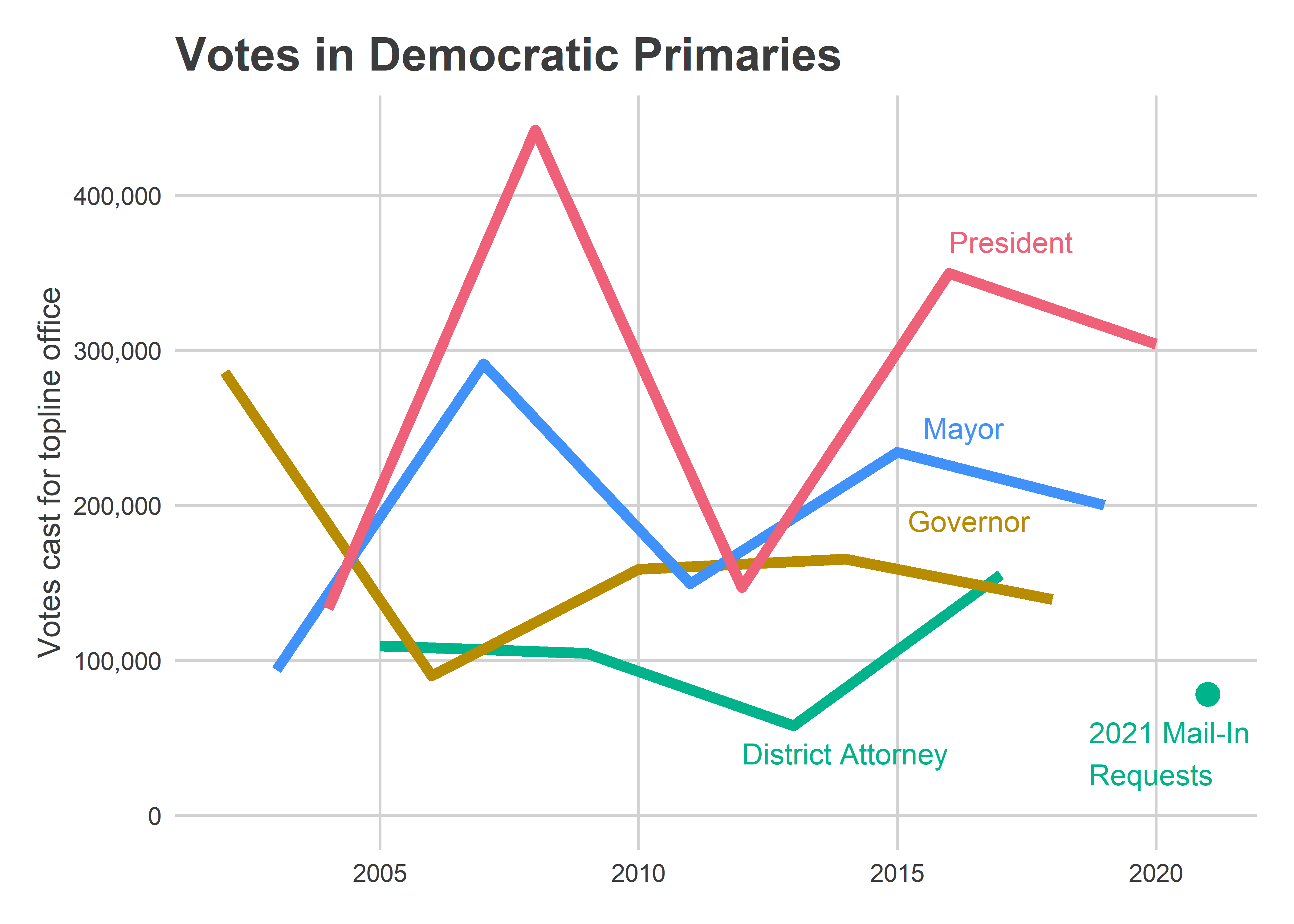
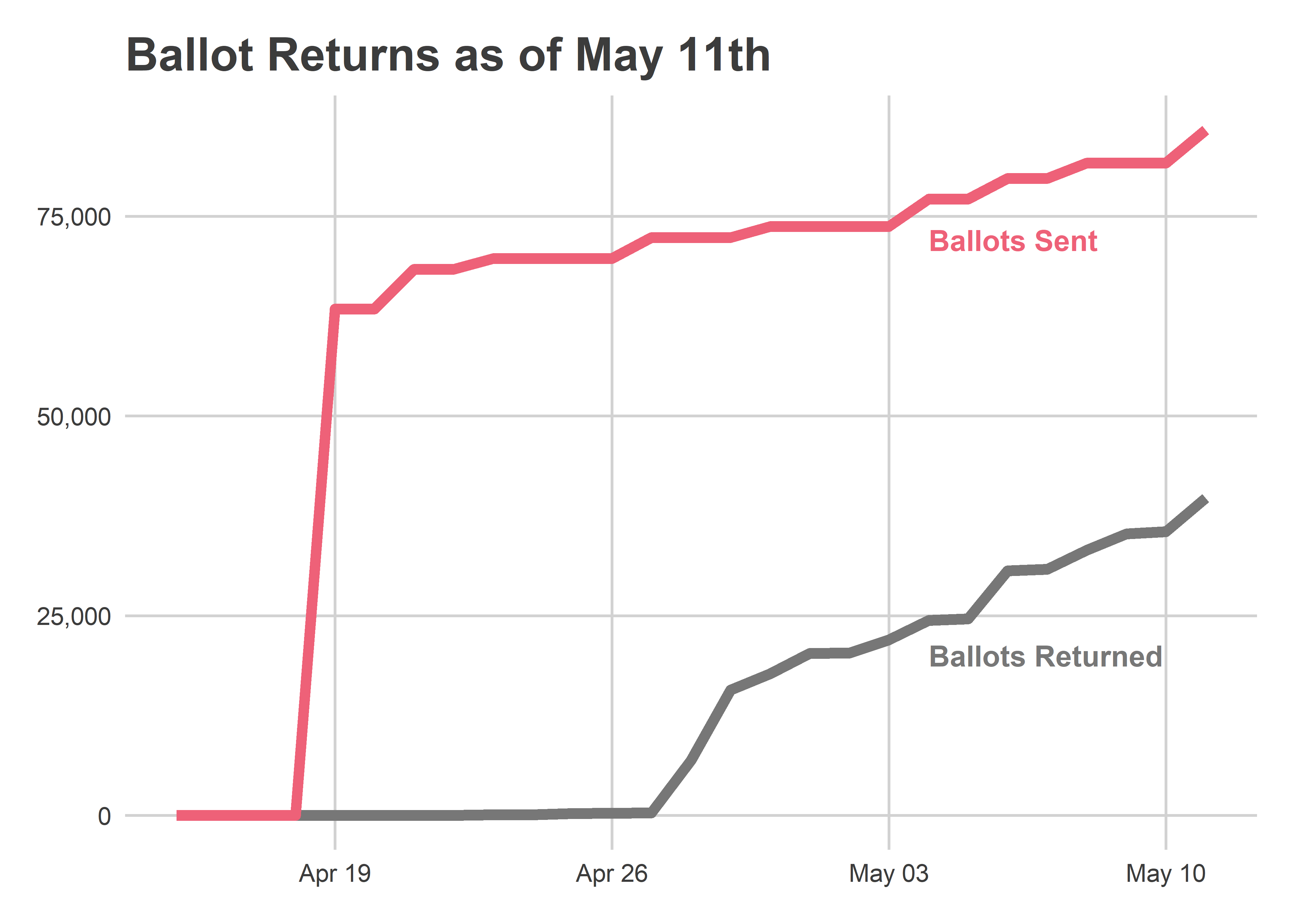
Mail in ballots appear about as proportional as last November (~50%). About 69,000 ballots have been requested, in an election where we might expect 150,000 voters (for context, 2017 saw 165K, but 2013, the last election with an incumbent DA, only saw 64K).

This also introduces interesting strategies for candidates. In an in-person election, the dramatic effect is getting literature in people’s hands at the polling place, via Ward endorsements or your own volunteers. But when half the voters vote at home, a campaign that can effectively target them the day they receive their ballot may get more bang for their buck.

You probably still don’t want to Bullet Vote.

Two years ago I published my polemic against casting a single vote when you’re allowed more, or “Bullet Voting”. This election gave me a clean example, and I want to try rephrasing it (to have a better link to point to).

In this election, you can vote for eight candidates. Suppose you have a single favorite, though. Should you only vote for them, to maximize their chance of winning?

No. 

(To be clear, there are definitely preferences that are compatible with that strategy. They’re just more extreme than you think.)

Suppose your favorite candidate is Michele Hangley, and your second is Nick Kamau. Assume that all candidates are equally likely to win (we can complicate this later). When would it make sense to only vote for Hangley, versus when should you vote for both Hangley and Kamau?

Notice that foregoing a vote for Kamau only makes Hangley more likely to win in a single situation: where Kamau is in 8th, and Hangley in 9th. But it hurts Kamau in fourteen situations: when Kamau is in 9th, and any of the other candidates is in 8th. Thus, foregoing your vote is only optimal if the difference in your preferences for Hangley and Kamau is fourteen times greater than the average difference between Kamau and everyone else. And he’s your second favorite!

Things change when you ask “Should I vote for seven candidates or eight?” Foregoing a vote for your eight favorite candidate–call them “H”–helps each of your 1st through 7th favorite candidates when they’re in 9th place overall and H is in 8th. But it helps H in all the cases where H is in 9th place and she’s losing to one of your 9th through 16th favorite candidates. So you should forego a vote for H whenever the average value difference between your top seven candidates and H is greater than 8/7 (1.14) the average value difference between H and everyone else, and vote for H if it’s less. That’s a lot closer.

In general, suppose you’ve voted for your favorite K-1 candidates, and are wondering if you should add a vote for your Kth? Doing so will hurt your 1st through (K-1)th candidates when they lose to K, but help your Kth favorite candidate when they’re losing to the remaining N-K candidates. So you should forego a vote for K when the average value difference between candidates 1, 2, …, K-1 and candidate K, is greater than (N-K)/(K-1) times the average value difference between candidate K and candidates K+1, K+2, …, N.

How would unequal win probabilities change this? Instead of just multiplying the counts of scenarios times the average preference differences, you would need to model the exact probability of each candidate finishing in 8th and 9th, and come up with an accurate difference in expected values among the strategies.

Philadelphia’s Changing Voting Blocs

In the past, I’ve relied heavily on what I call Philadelphia’s Voting Blocs, groups of Divisions that vote for similar candidates. These provide a simplified but extremely powerful way to capture broad geographic trends in candidates’ performance. They’re built on top of the same methodology that powers the Turnout Tracker and the Needle.

One thing that’s always bothered me is that I’ve assumed the Blocs were the same in 2002 as they are today. I wasn’t allowing the boundaries to change. As someone who literally has a Ph.D. in measuring the movement of emergent neighborhood boundaries, this is off brand.

Today, I’ll relax that assumption to fit a model that allows the Blocs to change over time.

The old, time-invariant Voting Blocs

First, here’s how the Blocs were modeled until today. The source data is a giant matrix with rows for each divisions and columns for each candidate from elections since 2002. I model the votes \(x_{ij}\) in division \(i\) for candidate \(j\) as \[ \log(E[x_{ij}]) = \log(T_{iy_j}) + \mu_j + U_i’DV_j \] where \(T_{ir_j}\) is the turnout in Division \(i\) for candidate \(j\)’s race (\(r_j\)), \(\mu_j\) is a candidate mean, \(U_i\) is a \(K\)-length vector of latent scores for division \(i\) (I’ll use \(K=3\)), \(V_j\) is a \(K\)-length vector of latent scores for candidates, and \(D\) is a \(K\) by \(K\) diagonal matrix of scaling factors. My original Voting Blocs I didn’t directly fit this, but instead calculated \(\hat{\mu_j}\) as the sample mean of \(\log(x_{ij}/T_{r_j})\) and then used SVD to calculate matrices \(U\), \(D\), and \(V\) on the residual.

The result was a set of latent scores for divisions and candidates: candidates with positive scores in a dimension did disproportionately well in divisions with a positive score in that dimension, and disproportionately poorly in divisions with a negative score (vice versa for candidates with negative scores, the sign is arbitrary).

Here are those dimensions:

View code
library(tidyverse)
library(sf)
library(magrittr)

# setwd("C:/Users/Jonathan Tannen/Dropbox/sixty_six/posts/svd_time/")

source("../../data/prep_data/data_utils.R", chdir=TRUE) # most_recent_file
source("../../admin_scripts/util.R")

PRESENT_VINTAGE <- "201911"
OFFICES <- c(
  "UNITED STATES SENATOR", "PRESIDENT OF THE UNITED STATES",
  "MAYOR", "GOVERNOR", "DISTRICT ATTORNEY", #"DISTRICT COUNCIL", 
  "COUNCIL AT LARGE", "CITY COMMISSIONERS"
)

df_raw <- most_recent_file("../../data/processed_data/df_major_") %>%
  readRDS() %>%
  mutate(warddiv = pretty_div(warddiv))

MIN_YEAR <- 2002 

df <- df_raw %>% 
  filter(
    candidate != "Write In",
    substr(warddiv, 1, 2) != "99", 
    (election_type == "primary" & substr(party, 1, 3) == "DEM") | election_type=="general", 
    office %in% OFFICES
  ) %>%
  filter(year >= MIN_YEAR) %>%
  group_by(year, election_type, warddiv, office) %>%
  mutate(total_votes = sum(votes)) %>%
  ungroup() %>%
  # filter(total_votes > 0) %>%
  mutate(
    pvote = votes / total_votes,
    candidate = factor(candidate),
    warddiv = factor(warddiv),
    year = asnum(year) - MIN_YEAR
  ) %>%
  group_by(year, election_type, office) %>%
  mutate(ncand = length(unique(candidate))) %>%
  filter(ncand > 1) %>%
  group_by(year, election_type, office, candidate) %>%
  # filter(n() > 1703) %>%
  ungroup()

df %<>%
  unite(candidate_key, office, candidate, party, year, election_type, remove=FALSE)

candidates <- df %>% 
  group_by(candidate_key, year) %>%
  summarise(
    pvote_city = sum(votes) / sum(total_votes),
    mean_log_pvote = mean(log(votes+1) - log(total_votes+ncand)),
    .groups="drop"
  )

df_wide <- df %>%
  left_join(candidates) %>%
  mutate(resid = log(votes + 1) - log(total_votes + ncand) - mean_log_pvote) %>%
  dplyr::select(candidate_key, warddiv, resid) %>%
  spread(key=candidate_key, value=resid)

mat <- as.matrix(df_wide %>% dplyr::select(-warddiv))
row.names(mat) <- df_wide$warddiv

mat[is.na(mat)] <- 0

K <- 3
svd_0 <- svd(mat, nu=K, nv=K)

U_0 <- data.frame(
  warddiv = row.names(mat),
  alpha = svd_0$u,
  beta = matrix(0, nrow=nrow(mat), ncol=K)
)

V_0 <- data.frame(
  candidate_key = colnames(mat),
  score=svd_0$v
) %>%
  left_join(candidates %>% dplyr::select(candidate_key, mean_log_pvote))

D_0 <- svd_0$d[1:K]
View code
divs <- st_read(
  sprintf("../../data/gis/warddivs/%s/Political_Divisions.shp", PRESENT_VINTAGE)
) %>%
  mutate(warddiv = pretty_div(DIVISION_N))map_u <- function(U, D, years=c(2002, 2020), dimensions=1:K){
  U_gg <-  U %>% 
    pivot_longer(cols=c(starts_with("alpha"), starts_with("beta"))) %>%
    separate(name,into=c("var", "num"), sep="\\.") %>%
    pivot_wider(names_from=var, values_from=value) %>%
    left_join(data.frame(num=as.character(dimensions), d=D)) %>%
    inner_join(
      as.data.frame(
        expand.grid(num = as.character(dimensions), year=years)
      )
    ) %>%
    mutate(val = (alpha + beta * (year-MIN_YEAR)) * d)
  
  ggplot(
    divs %>% left_join(U_gg)
  ) + 
    geom_sf(aes(fill=val), color=NA) + 
    scale_fill_gradient2("Dimension\nScore", low=strong_red, high=strong_blue) +
    facet_grid(num ~ year, labeller=labeller(.rows=function(x) sprintf("Dim %s", x))) +
    theme_map_sixtysix() %+replace% 
    theme(legend.position = c(1.5, 0.5), legend.justification="center") +
    ggtitle(title)
}

map_u(U_0, D_0, 2002) + ggtitle("SVD Results")

To those familiar with Philadelphia’s racial geography, Dimension 1 has clearly captured the White-Black political divide (or, similarly, the Democrtic-Republican one). It’s important to remember that the algorithm has no demographic or spatial information. Any spatial patterns or correlations with race are simply because those divisions vote for similar candidates.

The candidates who did disproportionately best in the red divisions are all Republicans: John McCain in 2008, Mitt Romney in 2012, Sam Katz in 2003. In Democratic primaries, the candidates who did disproportionately well were Hillary Clinton in 2008 and John O’Neill in 2017. Remember that this map adjusts for a candidate’s overall performance. So it’s not that John McCain won the red divisions, but that he did better than his citywide 16%.

Conversely, the candidates who did disproportionately best in the blue divisions were Chaka Fattah in the 2007 primary, Tariq Karim El-Shabazz in 2017, and Anthony Hardy Williams in 2015.

The second dimension is weaker than the first (as measured by \(D\) and exemplified as the weaker colors in the map). It captures candidates who did disproportionately well in Center City and the ring around it, and in Mount Airy and Chestnut Hill.

The candidates who did disproportionately best in the blue divisions were all third-party Council challengers: Andrew Stober in 2015, Nicolas O’Rourke in 2019, Kendra Brooks in 2019, and Kristin Combs in 2015. The candidates who did disproportionately best in the red divisions were John O’Neill and Michael Untermeyer in the 2017 DA primary and Ed Neilson in the 2015 Council primary.

The third dimension is the weakest, and has identified an interesting pattern: lumping together the Northwest, parts of the Northeast, and deep South Philly as blue, and Hispanic North Philly with Penn and other young sections of the city as red. This dimension has identified Democratic party power: the candidates who did disproportionately best in the blue divisions all had strong party backing, including Edgar Howard in the 2003 Commissioner primary, Allan Domb and Derek Green in the 2019 primary, and Jim Kenney in the 2011 primary. The candidates who did disproportionately best in the red divisions were non-party challengers (who didn’t align with Dimension 2’s progressive candidates): Nelson Diaz for 2015 mayor, Joe Vodvarka for 2010 senate, and third-party mayoral candidates Boris Kindij and Osborne Hart in 2015.

A fascinating note: remember that the model doesn’t know anything about space. There is nothing built into the model that tries to say neighboring divisions should have similar scores. All of the spatial correlations in the scores are purely because those divisions vote similarly.

Changes over time

All of the above I’ve discussed before. But the thing that’s bothered me is that these boundaries have all clearly changed since 2002. The base for progressive challengers has expanded into the ring around Center City: University City, Fishtown and Kensington, East Passyunk. And the demographics of the city have changed: we have a strongly growing Hispanic population, and Black householders continue to grow in Philadelphia’s Middle Neighborhoods. If you naively applied the boundaries from the maps above to a 2020 election, you would miss important shifts on the edges. We can do better.

Consider candidates who did well in each dimension, but from early and late in the data. Here are maps of some candidates that had large scores in the first:

View code
map_keys <- function(key_df){
  dim_1_map <- df %>% 
    inner_join(key_df) %>%
    arrange(sign, time) %>%
    mutate(
      candidate_key = factor(candidate_key, levels=unique(candidate_key)),
      votes=votes+1,
      total_votes=total_votes+ncand,
      pvote=votes/total_votes
    )
  
  dim_1_map %<>% 
    group_by(candidate_key) %>%
    mutate(
      pvote_city = sum(votes) / sum(total_votes)
    )
  
  winsorize <- function(x, pct=0.95){
    cutoff <- quantile(abs(x), pct, na.rm = T)
    replace <- abs(x) > cutoff 
    x[replace] <- sign(x[replace]) * cutoff
    x
  }
  
  ggplot(divs %>% left_join(dim_1_map)) +
    geom_sf(aes(fill=winsorize(log10(pvote / pvote_city))), color=NA) +
    scale_fill_viridis_c("log(\n % of Vote /\n % of Vote in city\n)") +
    facet_wrap(
      ~candidate_key, 2, 2, 
      labeller=labeller(
        candidate_key = function(key){
          candidate <- gsub(".*_(.*)_.*_(.*)_(.*)", "\\1", key) %>% format_name
          year <- as.integer(gsub(".*_(.*)_.*_(.*)_(.*)", "\\2", key)) + MIN_YEAR
          election <- gsub(".*_(.*)_.*_(.*)_(.*)", "\\3", key) %>% format_name
          sprintf("%s, %s %s", candidate, year, election)
        }
      )
    ) +
    theme_map_sixtysix() %+replace% theme(legend.position="right")
}

map_keys(
  tribble(
    ~candidate_key, ~sign, ~time,
    "MAYOR_SAM KATZ_REPUBLICAN_1_general", -1, 0,
    "PRESIDENT OF THE UNITED STATES_DONALD J TRUMP_REPUBLICAN_14_general", -1, 1,
    "MAYOR_JOHN F STREET_DEMOCRATIC_1_general", 1, 0,
    "MAYOR_ANTHONY HARDY WILLIAMS_DEMOCRATIC_13_primary", 1, 1
  )
) +
  ggtitle("Candidates with extreme scores in Dimension 1")

Notice that the boundaries in some places changed, such as Street’s performance in University City versus Hardy Williams’.

Here’s Dimension 2:

View code
map_keys(
  tribble(
    ~candidate_key, ~sign, ~time,
    "COUNCIL AT LARGE_KENDRA BROOKS_WORKING FAMILIES PARTY_17_general", -1, 1,
    "COUNCIL AT LARGE_ANDREW TOY_DEMOCRATIC_5_primary", -1, 0,
    "MAYOR_ROBERT A BRADY_DEMOCRATIC_5_primary", 1, 0,
    "DISTRICT ATTORNEY_JOHN O NEILL_DEMOCRATIC_15_primary", 1, 1
  )
) +
  ggtitle("Candidates with extreme scores in Dimension 2")

The main takeaway from the maps is that the Center City progressive bloc has expanded outward. Toy did better in a core Center City region, whereas Brooks outperformed to the West, South, and North of where he did. It’s a little hard to see, but Brady also won much more of Fishtown and Kensington than O’Neill did.

And finally, Dimension 3:

View code
map_keys(
  tribble(
    ~candidate_key, ~sign, ~time,
    "MAYOR_NELSON DIAZ_DEMOCRATIC_13_primary", -1, 1,
    "COUNCIL AT LARGE_JUAN F RAMOS_DEMOCRATIC_1_primary", -1, 0,
    "COUNCIL AT LARGE_KATHERINE GILMORE RICHARDSON_DEMOCRATIC_17_primary", 1, 1,
    "MAYOR_MICHAEL NUTTER_DEMOCRATIC_5_primary", 1, 0
  )
) +
  ggtitle("Candidates with extreme scores in Dimension 3")

Notice that the Hispanic cluster has expanded into the Northeast.

Time-varying Blocs

Instead of the static model, consider a model where divisions’ scores are allowed to change over time. \[ \log(E[x_{ij}]) = \log(T_i) + \mu_j + (\alpha_i + \beta_i y_j)’DV_j \] where \(\alpha_i + \beta_i y_j\) is a linearly changing vector of division \(i\)’s scores by year \(y\). We’ve now allowed the embedding of the Divisions in University City, for example, to become more positive in the progressive Dimension 2 from 2002 to 2020.

Fitting this model isn’t as easy as SVD. I’ll use gradient descent to find a maximum likelihood solution, initialized with the time-invariant SVD solution. Since I’m now using likelihood, I’ll also assume a poisson distribution for \(x\). [One mathematical note: we lose the guarantee of SVD that the U- and V-vectors will be orthogonal. I’m not really worried about this, and am not convinced there are practical implications as long as we sufficiently normalize, but be forewarned.]

View code
VERBOSE <- TRUE
printv <- function(x, ...) if(VERBOSE) print(x, ...=...) 

U_df <- U_0
V_df <- V_0
D <- D_0

update_U <- function(df, D, V_df){
  form <- sprintf(
    "votes ~ -1 + %s",
    paste(sprintf("dv.%1$i + year:dv.%1$i", 1:K), collapse=" + ")
  )
  
  for(k in 1:K){
    var.k <- function(stem) sprintf("%s.%i", stem, k)
    V_df[[var.k("dv")]] <- D[k] * V_df[[var.k("score")]] 
  }
  
  U_new <- df %>% 
    mutate(votes=round(votes)) %>%
    left_join(
      V_df %>% select(candidate_key, mean_log_pvote, starts_with("dv.")), 
      by=c("candidate_key")
    ) %>%
    filter(total_votes > 0) %>%
    group_by(warddiv) %>%
    do(
      broom::tidy(
        glm(
          as.formula(form), 
          data = ., 
          family=poisson(link="log"),
          offset=log(total_votes) + mean_log_pvote
        )
      ) 
    ) %>% 
    ungroup()
  
  U_new %<>%
    mutate(
      term_clean=case_when(
        grepl("year", term) ~ gsub(".*dv\\.([0-9]+)(:.*|$)", "beta.\\1", term),
        TRUE ~ gsub("dv\\.([0-9]+)$", "alpha.\\1", term)
      )
    ) %>%
    select(warddiv, term_clean, estimate) %>%
    spread(key=term_clean, value=estimate)
  
  return(U_new)
}


update_V <- function(df, U_df, D){
  
  dfu <- df %>% 
    left_join(U_df,by="warddiv")
  
  for(k in 1:K){
    var.k <- function(stem) sprintf("%s.%i", stem, k)
    dfu[[var.k("du")]] <- D[k] * (dfu[[var.k("alpha")]] + dfu[[var.k("beta")]] * dfu$year)
  }
  
  form <- sprintf(
    "votes ~ 1 + %s",
    paste(sprintf("du.%1$i", 1:K), collapse=" + ")
  )
  
  V_new <-  dfu %>%
    mutate(votes=round(votes)) %>%
    filter(total_votes > 0) %>%
    group_by(candidate_key) %>%
    do(
      broom::tidy(
        glm(
          as.formula(form), 
          data = .,
          family=poisson(link="log"),
          offset=log(total_votes)
        )
      ) 
    ) %>% 
    mutate(
      term = case_when(
        grepl("^du", term) ~ gsub("^du", "score", term),
        term=="(Intercept)" ~ "mean_log_pvote"
      )
    ) %>%
    select(candidate_key, term, estimate) %>%
    spread(key=term, value=estimate)
  
  return(V_new)
}

scale_udv <- function(U_df, D, V_df){
  for(k in 1:K){
    var.k <- function(stem) paste0(stem, ".", k)
    
    sum_sq <- sum(V_df[[var.k("score")]]^2)
    D[k] <- D[k] * sqrt(sum_sq)
    V_df[[var.k("score")]] <- V_df[[var.k("score")]] / sqrt(sum_sq)
    
    u <- U_df[[var.k("alpha")]] + outer(U_df[[var.k("beta")]], 0:max(df$year))
    sum_sq <- sum(u^2)
    D[k] <- D[k] * sqrt(sum_sq)
    U_df[[var.k("alpha")]] <- U_df[[var.k("alpha")]] / sqrt(sum_sq)
    U_df[[var.k("beta")]] <- U_df[[var.k("beta")]] / sqrt(sum_sq)
  }
  
  return(list(U=U_df, D=D, V=V_df))
}


predict_score <- function(df, U_df, V_df, D){
  outer <- df %>%
    select(warddiv, candidate_key, year, votes, total_votes) %>%
    left_join(U_df, by="warddiv") %>%
    left_join(V_df, by=c("candidate_key"))
  
  vec <- 0
  for(k in 1:K){
    var.k <- function(var) paste0(var, ".", k)
    a <- outer[[var.k("alpha")]]
    b <- outer[[var.k("beta")]]
    u <- (a + b*outer$year)
    v <- outer[[var.k("score")]]
    vec <- vec +  u * v * D[k]
  }
  
  outer$udv <- vec
  outer$log_pred <- outer$mean_log_pvote + log(outer$total_votes) + outer$udv
  outer$pred <- exp(outer$log_pred)
  outer$resid <- outer$votes - outer$pred
  return(outer %>% select(candidate_key, warddiv, udv, votes, pred, log_pred, resid, year))
}

calc_ll <- function(pred){
  sum(
    dpois(round(pred$votes), pred$pred, log=TRUE)[df$total_votes > 0]
  )
}

pred_0 <- predict_score(df, U_0, V_0, D_0)
resids <- calc_ll(pred_0)

RUN <- FALSE
if(RUN){
  for(i in 1:100){
    U_df <- update_U(df, D, V_df)
    new_pred <- predict_score(df, U_df, V_df, D)
    # plot_compare_to_svd(new_pred)
    printv(
      sprintf("%i U: %0.6f", i, calc_ll(new_pred))
    )
    resids <- c(resids, calc_ll(new_pred))
    
    V_df <- update_V(df, U_df, D)
    new_pred <- predict_score(df, U_df, V_df, D)
    # plot_compare_to_svd(new_pred)
    printv(
      sprintf("%i V: %0.6f", i, calc_ll(new_pred))
    )
    resids <- c(resids, calc_ll(new_pred))
    
    ## Not necessary to model D, since V is always maximized. Instead, just rescale it.
    # D <- update_D(df, U_df, V_df)
    scaled <- scale_udv(U_df, D, V_df)
    U_df <- scaled$U
    D <- scaled$D
    V_df <- scaled$V
    
    new_pred <- predict_score(df, U_df, V_df, D)
    # plot_compare_to_svd(new_pred)
    printv(
      sprintf("%i D: %0.6f", i, calc_ll(new_pred))
    )
    if(abs(calc_ll(new_pred)-resids[length(resids)]) > 1e-8) 
      stop("D changed resids, it shouldn't.")
    plot(log10(diff(resids)), type="b")
  }
  
  res <- list(U=U_df, D=D, V=V_df)
  saveRDS(res, file=dated_stem("svd_time_res", "", "RDS"))
} else {
  res <- readRDS(max(list.files(pattern="svd_time_res")))
  U_df <- res$U
  V_df <- res$V
  D <- res$D
}
View code
## Just for fun, I figured I'd try the model in the new R torch package too :)

if(RUN){
  library(torch)  
  
  V_t <- torch_tensor(
    as.matrix(V_df %>% ungroup() %>% select(starts_with("score"))),
    requires_grad=TRUE
  )
  cand_means <- torch_tensor(V_df$mean_log_pvote, requires_grad=TRUE)
  
  alpha <- torch_tensor(
    as.matrix(U_df %>% select(starts_with("alpha"))), 
    requires_grad=TRUE
  )
  beta <- torch_tensor(
    as.matrix(U_df %>% select(starts_with("beta"))), 
    requires_grad=TRUE
  )

  year <- torch_tensor(t(t(df$year)), requires_grad=FALSE)
  
  # Don't let D change, since V will scale freely.
  D_t <- torch_tensor(D[1:K], requires_grad=FALSE)

  
  cands_i <- match(df$candidate_key, V_df$candidate_key)
  divs_i <- match(df$warddiv, U_df$warddiv)
  
  votes <- torch_tensor(df$votes, requires_grad=FALSE)
  log_total_votes <- torch_tensor(df$total_votes, requires_grad=FALSE)$log()
  
  valid_rows <- df$total_votes > 0
  
  create_dfs <- function(alpha, beta, D, V, cand_means){
      U_df <- data.frame(
        warddiv=U_df$warddiv,
        alpha=as_array(alpha),
        beta=as_array(beta)
      )
      
      V_df <- data.frame(
        candidate_key=V_df$candidate_key,
        score=as_array(V),
        mean_log_pvote=as_array(cand_means)
      )
      
      return(scale_udv(U_df, as_array(D), V_df))
  }
  
  cand_rows <- lapply(candidates$candidate_key, function(x) which(df$candidate_key == x))
  
  learning_rate <- 1e-4
  lls <- c()
  for (t in seq_len(5e3)) {
    alpha_i <- alpha[divs_i]
    beta_i <- beta[divs_i]
    cand_means_i <- cand_means[cands_i]
    V_i <- V_t[cands_i,]
    
    udv <- (alpha_i + beta_i$mul(year))$mul(D_t)$mul(V_i)$sum(2)
    log_pred <- cand_means_i$add(log_total_votes)$add(udv)

    loss <- nn_poisson_nll_loss()
    ll <- loss(
      log_pred[valid_rows],
      votes[valid_rows]
    )
    
    ll$backward()
    
    if (t %% 100 == 0 || t == 1){
      with_no_grad({
        lls <- c(lls, as.numeric(ll))
        cat("Step:", t, ":\n", as.numeric(ll), "\n")
        
        dfs <- create_dfs(alpha, beta, D_t, V_t, cand_means)
        new_pred <- predict_score(df, dfs$U, dfs$V, dfs$D)
        resids <- c(resids, calc_ll(new_pred))
        plot(log10(diff(resids)), type="b")
        cat(tail(resids, 1), "\n")
      })
    }
    
    if(is.na(as.numeric(ll))) stop("Bad ll")
    
    with_no_grad({
      V_t$sub_(learning_rate * V_t$grad)
      cand_means$sub_(learning_rate * cand_means$grad)
      alpha$sub_(learning_rate * alpha$grad)
      beta$sub_(learning_rate * beta$grad)
      
      # D$sub_(learning_rate * D$grad)
      
      V_t$grad$zero_()
      cand_means$grad$zero_()
      alpha$grad$zero_()
      beta$grad$zero_()
      # D$grad$zero_()
      
    })
  }
  
  res <- create_dfs(alpha, beta, D_t, V_t, cand_means)
  U_df <- res$U
  D <- res$D
  V_df <- res$V
  saveRDS(res, file=dated_stem("svd_time_res", "", "RDS"))
}

The results show how the dimensions have changed over time.

View code
# V_df %>% 
#   # filter(grepl("_primary", candidate_key)) %>%
#   arrange(-score.3)

map_u(U_df, D, c(2002, 2020)) + ggtitle("Time-Varying Results")

The first dimension, which I said captures Black-White divides (or, similarly, Democratic-Republican), shows that the blue dimension has expanded in the Northwest and in Overbrook/Wynnefield, while the red dimension have expanded outward from its dense Center City core, and lost ground in the lower Northeast. John Street did disproportionately well in the blue divisions in 2003, while Tariq El-Shabazz did disproportionately well in 2017. Meanwhile, the candidates who did disproportionately best in the red dimension are Republicans: John McCain, Mitt Romney, Sam Katz.

The second dimension, for which I said blue captures progressive candidates, has expanded outward even more from Center City, now covering much of Fishtown and Kensington, upper South Philly, and into Brewerytown. Meanwhile, the wealthy progressive base in Wynnefield and Overbrook is gone, having been replaced by the strong-Democrat dimension 1.

The third dimension is hard to figure out. In 2002, It was strongly red in Hispanic North Philly, deep South Philly, and Overbrook. By 2020, it’s broadly red in Hispanic North Philly up into the lower Northeast. Meanwhile, the blue divisions include the Northeast and the Northwest. The General election candidates who do disproportionately well in the red divisions are third parties–Osborne Hart and John Staggs in 2015, Neal Gale in 2018–and the candidates who do well in the Democratic Primary typically have Hispanic surnames–Nelson Diaz in 2015, Humberto Perez in 2011, Deja Lynn Alvarez in 2019. Remember, this is all after controlling for the stronger dimensions 1 and 2, and is not a terribly influential dimension.

Changing Voting Blocs

The Voting Blocs themselves were a discretized version of these continuous scores into four categories.

In previous iterations, I hand-curated the Voting Blocs by choosing cutoffs for the categories. Now, since we have different scores across different years, I’ll try to automate it. I’ll use simple K-means clustering on the scores.

View code
years <- c(2002, 2020)

mutate_add_score <- function(U_df, D, year, min_year=MIN_YEAR){
  year_dm <- year - min_year
  for(k in 1:K){
    var.k <- function(x) sprintf("%s.%i", x, k)
    U_df[[var.k("score")]] <- D[k] * (
      U_df[[var.k("alpha")]] + U_df[[var.k("beta")]] * year_dm
    )
  }
  return(U_df)
}

div_cats <- purrr::map(
  c(2002, 2020), 
  function(y) mutate_add_score(U_df, D, as.integer(y))
) %>%
  bind_rows(.id = "id") %>%
  mutate(year = c(2002, 2020)[as.integer(id)])

# plot(div_cats %>% select(starts_with("score")))
  
km <- kmeans(
  div_cats[, c("score.1","score.2","score.3")], 
  centers=matrix(
    10 * c(
      1, -1, 0, 
      -1, 1, 0, 
      0, -1, -1, 
      -1, -1, 1
    ), 
    4, 3, 
    byrow=T
  )
)

cats <- c(
  "Black Voters",
  "Wealthy Progressives",
  "Hispanic Voters",
  "White Moderates"
)
div_cats$cluster <- factor(cats[km$cluster], levels=cats)
cat_colors <- c(light_blue, light_red, light_orange, light_green)
names(cat_colors) <- cats  

plot(div_cats %>% select(starts_with("score")), col=cat_colors[km$cluster])

The three score dimensions are chopped into four groups. Bloc 1 (Blue), has positive scores in Dimension 1. These are the Black Voter divisions. Bloc 2 (Red) has middling scores in Dimension 1 but positive scores in Dimension 2. These are the Wealthy Progressive divisions. Bloc 3 has middling scores in Dimension 1, negative scores in Dimension 2, and negative scores in Dimension 3. These are the Hispanic Voter divisions. (I previously called these Hispanic North Philly, but once we allow for time, it turns out that some South Philly divisions in 2002 were also in the group). Bloc 4 has negative scores in Dimension 1 and negative scores in Dimension 2. These are the White Moderate divisions.

View code
ggplot(divs %>% left_join(div_cats)) +
  geom_sf(aes(fill=cluster), color=NA) +
  scale_fill_manual(NULL, values=cat_colors) +
  facet_wrap(~year) +
  theme_map_sixtysix() %+replace%
  theme(legend.position="bottom", legend.direction="horizontal") +
  ggtitle("Voting Blocs over time")

In the maps above, you can clearly see the expansion of the Wealthy Progressive divisions outward from Center City, and growth of the Black Voter divisions in North and West Philly, along with a shift in the Hispanic Voter divisions eastward and up into the lower Northeast.

With the moving boundaries, the changes in Blocs’ share of the vote is even starker than before.

View code
mutate_add_cat <- function(U_df, D, year, km, min_year=MIN_YEAR){
  U_score <- mutate_add_score(U_df, D, year, min_year)
   
  cluster <- apply(
    as.matrix(km$centers),
    1,
    function(center) {
      apply(
        as.matrix(U_score %>% select(starts_with("score"))),
        1,
        function(row) sum((row - center)^2)
      )
    }
  )
  
  cat <- cats[apply(cluster, 1, which.min)]
  
  return(U_score %>% mutate(cat=cat))
}

div_cats <- purrr::map(
  2002:2020, 
  function(y) mutate_add_cat(U_df, D, as.integer(y), km)
) %>% bind_rows(.id = "id") %>% mutate(year=as.integer(id)-1)

turnout_df <- df %>% 
  filter(is_topline_office) %>%
  group_by(year, election_type, warddiv) %>%
  summarise(turnout=sum(votes), .groups="drop") %>%
  left_join(div_cats) %>%
  group_by(year, election_type) %>%
  do(
    mutate_add_cat(U_df=., D=D, year=.$year + MIN_YEAR, km=km)
  )

turnout_cat <- turnout_df %>% 
  group_by(year, election_type, cat) %>%
  summarise(turnout=sum(turnout)) %>%
  group_by(year, election_type) %>%
  mutate(prop=turnout/sum(turnout))

ggplot(
  turnout_cat, 
  aes(x=year+MIN_YEAR, y=100*prop, color=cat)
) +
  geom_line(aes(linetype=election_type), size=2)+
  geom_text(
    data=tribble(
      ~prop, ~cat,
      0.48, "Black Voters",
      0.35, "Wealthy Progressives",
      0.21, "White Moderates",
      0.06, "Hispanic Voters"
    ),
    aes(label=cat),
    fontface="bold",
    x=2015.5,
    hjust=0
  ) +
  scale_color_manual(values=cat_colors, guide=FALSE) +
  theme_sixtysix() +
  expand_limits(y=0, x=2021) +
  labs(
    title="Voting Blocs' proportions of turnout",
    subtitle="Grouped by changing blocs",
    y="Percent of Turnout",
    x=NULL,
    linetype=NULL
  )

Black Voters have seen an increasing share of the turnout since 2002, though that’s somewhat mitigated by changes since 2016. Wealthy Progressive share took a clear leap in 2017 and after. White Moderate and Hispanic Voter shares have seen a steady decline since 2002. Notice that this is not directly applicable to people; this is all traits of divisions. For example, if the Hispanic population is becoming more dispersed across the city, or voting more similarly to the other Voting Blocs, they may represent a steadier share of the electorate even while Divisions clearly identifiable as Hispanic Voters are sparser. This is an instance of what is known as Ecological Inference.

Next Steps

I’ll be adapting all of my tooling: the Turnout Tracker, Election Needle, and the Voting Blocs, to use these time-varying dimensions instead. To come!