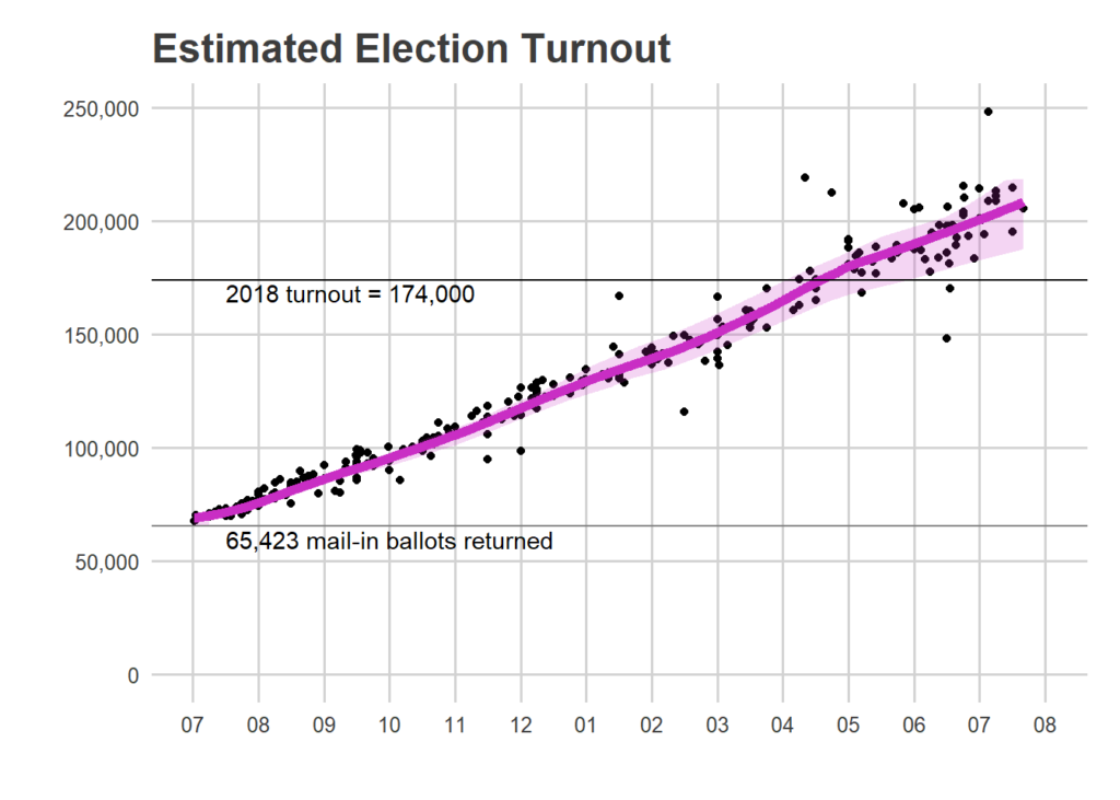
Will straight-ticket’s elimination hurt Dem judges?

November 2nd will bring Pennsylvania’s municipal elections. In Philadelphia, Larry Krasner will certainly win. However, there are several state judicial races on the ballot, including for the Supreme Court. The court is represented currently by five Democrats and two Republicans, a balance that led to its anti-gerrymandering ruling.

The 2019 election reform bill that created no-excuse vote by mail (in Covid hindsight, a small miracle) also removed straight-party voting, in which a voter could vote for all Democratic or Republican candidates with the push of a single button.

This was expected to hurt Democratic judges downballot, as voters would vote for topline races but leave lower ones blank. An analysis by PennLive found that over 1/3 of voters used the straight-ticket button, and it was used disproportionately by Democrats.

We’ve had one general election since the law went into effect, so I thought I’d see if we could say anything about that ahead of next Tuesday’s race.

Downballot Results

In a typical judicial election, Philadelphia casts about 10% of the votes. Philadelphia’s four suburban counties–Bucks, Chester, Delaware, and Montgomery–cast an additional 26% in recent years. (I’m using Superior Court elections, which are more consistent that Supreme Court.)

View code
library(tidyverse)
devtools::load_all("../../admin_scripts/sixtysix/")

election_files <- list.files("../../data/pa_election_data/electionreturns.pa.gov", pattern = "PA_Official_[0-9]+_general", full.names = TRUE)

dfs <- list()
for(file in election_files){
  dfs[[file]] <- read_csv(file)
}
df <- bind_rows(dfs)
names(df) <-
  gsub(" ", "_", 
       gsub(" name$", "", tolower(names(df)))
  )
df$year <- as.numeric(substr(df$election, 1, 4))

counties <- df %>%
  filter(year == "2020", office == "President of the United States") %>%
  select(county, candidate, votes) %>%
  pivot_wider(names_from=candidate, values_from=votes) %>%
  mutate(pdem_2020 = `BIDEN, JOSEPH ROBINETTE JR` / (`BIDEN, JOSEPH ROBINETTE JR` + `TRUMP, DONALD J.`)) %>%
  mutate(cat = case_when(
    county == "PHILADELPHIA" ~ "Philadelphia",
    county %in% c("MONTGOMERY", "BUCKS", "CHESTER", "DELAWARE") ~ "Philadelphia Suburbs",
    TRUE ~ "Rest of PA"
  ))

cat_colors <- c(
  Philadelphia = colors_sixtysix()$strong_red, 
  `Philadelphia Suburbs` = colors_sixtysix()$strong_green,
  `Rest of PA` = colors_sixtysix()$strong_blue
)
  
judge_results <- df %>% 
  filter(
    office %in% c("Judge of the Superior Court")
    # ifelse(
    #   year %% 4 == 1,
    #   office %in% c("Justice of the Supreme Court"),
    #   office %in% c("Judge of the Superior Court")
    # )
  ) %>% 
  group_by(county, year) %>%
  summarise(
    ndem = length(unique(candidate[substr(party, 1, 3) == "Dem"])),
    total_votes = sum(votes),
    dem_votes = sum(votes * (substr(party, 1, 3) == "Dem")),
    rep_votes = sum(votes * (substr(party, 1, 3) == "Rep"))
  ) %>%
  left_join(counties)

judge_cats <- judge_results %>% group_by(cat, year) %>%
  summarise(dem_votes=sum(dem_votes), rep_votes=sum(rep_votes)) %>%
  mutate(
    total_2party=dem_votes + rep_votes,
    pdem = dem_votes/ total_2party
  ) %>%
  group_by(year) %>%
  mutate(prop_of_year = total_2party / sum(total_2party))

ggplot(
  judge_cats,
  aes(x = year, y=100*prop_of_year)
) +
  geom_point(aes(color=cat), size=2)+
  geom_line(aes(group=cat, color=cat), size=1) +
  expand_limits(y=0) +
  theme_sixtysix() +
  geom_text(
    data=tribble(
      ~x, ~y, ~cat,
      2019, 7, "Philadelphia",
      2019, 32, "Philadelphia Suburbs",
      2019, 73, "Rest of PA"
    ),
    aes(x=x, y=y, label=cat, color=cat),
    hjust=1,
    fontface="bold"
  ) +
  scale_color_manual(guide=FALSE, values=cat_colors) +
  labs(
    title="Philadelphia casts about 10% of Judicial votes",
    subtitle="Elections for Superior Court",
    y="Percent of votes cast",
    x=NULL
  )

With that 10%, Philadelphia is by far more Democratic than the rest of the state. Democratic candidates receive over 80% of the vote here. The suburbs are significantly more Democratic recently, at 56% in recent years, and the rest of the state is becoming more Republican fast (53% in 2017, then 57% in 2019).

View code
ggplot(
  judge_cats,
  aes(x=year, y=100*pdem)
) + 
  geom_point(aes(color=cat), size=2)+
  geom_line(aes(group=cat, color=cat), size=1) +
  expand_limits(y=0) +
  theme_sixtysix() +
  geom_text(
    data=tribble(
      ~x, ~y, ~cat,
      2019, 78, "Philadelphia",
      2019, 62, "Philadelphia Suburbs",
      2019, 40, "Rest of PA"
    ),
    aes(x=x, y=y, label=cat, color=cat),
    hjust=1,
    fontface="bold"
  ) +
  scale_color_manual(guide=FALSE, values=cat_colors) +
  labs(
    title="Philadelphia votes over 80% Democratic",
    subtitle="Elections for Superior Court",
    y="Percent cast for Democrats",
    x=NULL
  )

I don’t have the actual straight-ticket use numbers. Instead, let’s look at downballot vote rates. Since 2011 Philadelphia has cast about 90% of the votes for Superior Court candidates as it has for topline races.

View code
df_phila <- readRDS("../../data/processed_data/df_major_type_20210118.Rds")
df_phila <- df_phila %>%  filter(election_type=="general")

ndem <- df_phila %>%
  filter(office == "JUDGE OF THE SUPERIOR COURT", substr(party, 1, 3) == "DEM") %>%
  group_by(year) %>%
  summarise(ndem = length(unique(candidate)))

vpv_phila <- df_phila %>% 
  filter(
    asnum(year) %% 2 == 1,
    is_topline_office | (office == "JUDGE OF THE SUPERIOR COURT")
  ) %>%
  mutate(isjudge = ifelse(office == "JUDGE OF THE SUPERIOR COURT", "Sup Court", "Topline")) %>%
  group_by(year, isjudge) %>%
  summarise(votes=sum(votes)) %>%
  pivot_wider(names_from=isjudge, values_from=votes) %>%
  left_join(ndem) %>%
  mutate(
    votes_per_voter = `Sup Court` / (ndem * Topline)
  )
  
ggplot(
  vpv_phila %>% filter(year != 2005),
  aes(x=asnum(year), y=100*votes_per_voter)
) + 
  geom_point() +
  geom_path() +
  labs(
    title="90% of Philadelphian voters vote for judges",
    y="Votes for Superior Court / \n(Topline Votes * N(Vacancies)) (%)",
    x=NULL
  ) +
  scale_y_continuous(breaks = seq(0, 100, 10)) +
  expand_limits(y=50:100)+
  theme_sixtysix()

I can’t create the same plot across the state because the PA results don’t provide municipal races. But here’s that plot for even years, using State Rep votes as the numerator.

View code
county_votes_presgov <- df %>% 
  filter(
    office %in% c("President of the United States", 'Governor')
  ) %>%
  group_by(year, county) %>%
  summarise(votes_presgov=sum(votes))

county_votes_strep <- df %>% 
  filter(
    office %in% c("Representative in the General Assembly")
  ) %>%
  group_by(year, county) %>%
  summarise(votes_strep=sum(votes))

votes_strep <- county_votes_strep %>%
  left_join(county_votes_presgov) %>%
  left_join(counties) %>%
  group_by(cat, year) %>%
  summarise(
    across(c(votes_presgov, votes_strep), sum)
  )

ggplot(
  votes_strep,
  aes(x=year, y=100*votes_strep / votes_presgov, color=cat)
) +
  geom_point() +
  geom_line(aes()) +
  expand_limits(y=c(50,100)) +
  scale_y_continuous(breaks = seq(0, 100, 10)) +
  scale_color_manual(guide=FALSE, values=cat_colors) +
  theme_sixtysix() +
  geom_text(
    data=tribble(
      ~x, ~y, ~cat,
      2020, 85, "Philadelphia",
      2020, 100, "Philadelphia Suburbs",
      2020, 95, "Rest of PA"
    ),
    aes(x=x, y=y, label=cat, color=cat),
    hjust=1,
    fontface="bold"
  ) +
  labs(
    title="Philadelphia's downballot rate dropped in 2020",
    y="Votes for State Rep / Votes for Topline (%)",
    x=NULL
  )

There’s serious variance across years, as some elections draw only super-voters, while others draw only topline voters. But something big happened in 2020: Philadelphia’s ratio plummeted, while the rest of the state *increased*. It’s not entirely clear what might have caused this. It could certainly be the elimination of straight-ticket voting. It could also be an influx of lower-propensity voters, who are less likely to vote downballot, or even a signal of distaste for the Democratic party (a costless signal, since most of these races were non-competitive).

This change was completely different between mail and Election Day voters. Among Philadelphia’s mail voters, State Rep votes were at 91.5% of Presidential votes. Among Election Day voters, that was only 83%. There is obviously a ton of omitted variable bias in this difference–mail-in voters were different in many ways from Election Day voters–but it’s at least suggestive that maybe the physical experience of mail-in ballots makes voters more likely to vote downballot.

We might worry that this drop would not just hurt Philadelphia, but other Democratic counties. But there does not appear to be a broad correlation between Democratic vote share and changes in downballot vote rates.

View code
county_vpv_scatter <- county_votes_strep %>%
  left_join(county_votes_presgov) %>%
  left_join(counties) %>%
  filter(year %in% c(2018, 2020)) %>%
  mutate(vpv=votes_strep / votes_presgov) %>%
  group_by(county) %>%
  mutate(votes_20 = votes_presgov[year==2020]) %>%
  select(year, county,cat, vpv, pdem_2020, votes_20) %>%
  pivot_wider(
    names_from=year, values_from=vpv
  ) %>%
  mutate(ratio = `2020`/`2018`) 

ggplot(county_vpv_scatter, aes(x=100*pdem_2020, y=ratio)) +
  geom_smooth(weights="votes_20", color="grey60") +
  geom_point(aes(size=votes_20, color=cat)) +
  geom_hline(yintercept=1) +
  theme_sixtysix() +
  scale_size_area(guide=FALSE)+
  scale_color_manual(guide=FALSE, values=cat_colors) +
  labs(
    title="No clear trend in downballot vote changes",
    subtitle="Change in voting rates for State Rep, 2018-2020.",
    y="2020 Votes per Voter / 2018 Votes per Voter\n(Votes per Voter = State Rep Votes / Topline Votes)",
    x="2020 Percent for Biden"
  )

Will Philadelphia’s drop continue this year?

This election is entirely different from last November, obviously. We’re entering the lowest turnout election in the four-year cycle, down from 2020’s highest. A surge in low-interest voters would have made this rate low in 2020, as those hard-to-get voters are also less likely to vote for non-Presidential races. Also, State Representative races are differentially competitive across the state. Add Covid, the novelty of mail-in voting, and Philadelphia’s new voting machines, and it’s not clear how generalizable 2020’s patterns will be to this year. (and as @Dan_UA points out, Supreme Court is not literally downballot ; so it depends if you think the mechanism is literal ballot position or voter interest.)

Suppose this trend did continue this year, though. Would it have mattered? In 2017, Republican Sally Mundy beat out Democrat Dwayne Woodruff by 95,000 votes. In that race, 200,000 Philadelphians voted. The 5% drop in downballot votes above would mean 10,000 votes, of which we’d expect Democrats to net 6,000. So it wouldn’t have affected 2017, but might in a much tighter race.

Redistricting Council

With the release of 2020’s Census data, redistricting will kick into gear. While boundaries for both the US Congress and State Senate and House will be redrawn, I thought I’d start close to home: City Council.

Philadelphia’s City Council consists of 17 seats, 10 of which are districted and the rest At Large. For the drawing of those 10 districts, the primary restriction imposed by the Charter is that they must have relatively equal populations. This has been implemented as each district being within 5% of one tenth of the city’s total population. Council has six months from the release of the data to produce maps, which would put the deadline at March 12, though that might depend on resolution of the allocation of incarcerated people.

I’ll use my jaywalkr library to crosswalk the data.

Methodological Note: I haven’t adapted the crosswalking for the Census’ Differential Privacy. It shouldn’t make a huge difference when aggregated to council districts. For the later analyses, I’ll use Block Groups which are less affected than Blocks.

View code
library(sf)
library(dplyr)
library(ggplot2)
library(readr)
library(tidyr)
devtools::load_all("../../admin_scripts/sixtysix/")

bgs <- st_read("../../data/gis/census/tl_2020_42_bg/tl_2020_42_bg.shp", quiet=TRUE) %>%
  filter(COUNTYFP == "101")

council <- st_read("../../data/gis/city_council/Council_Districts_2016.shp", quiet=TRUE)
council <- st_transform(council, st_crs(bgs))

blocks <- st_read(
  "../../data/gis/census/tl_2020_42101_tabblock/tl_2020_42101_tabblock20.shp", 
  quiet=TRUE
)

block_pops <- read_csv(
  "../../data/census/decennial_2020_poprace_phila_blocks/DECENNIALPL2020.P4_data_with_overlays_2021-09-22T083940.csv",
  skip=1
)

block_pops <- block_pops %>% rename(total_pop = `!!Total:`) %>% select(id, total_pop) 
block_pops <- block_pops %>% mutate(GEOID20 = substr(id, 10, 25))

blocks <- blocks %>% left_join(block_pops, by="GEOID20")
block_centroids <- st_centroid(blocks) %>% filter(total_pop > 0)

bg_pops <- read_csv(
  "../../data/census/decennial_2020_poprace_phila_bg/DECENNIALPL2020.P2_data_with_overlays_2021-09-21T090431.csv", 
  skip=1
) %>%
  mutate(GEOID = substr(id, 10, 25))

bg_pops <- bg_pops %>%
  mutate(
    total_pop = `!!Total:`,
    hispanic = `!!Total:!!Hispanic or Latino`,
    black = `!!Total:!!Not Hispanic or Latino:!!Population of one race:!!Black or African American alone`,
    white = `!!Total:!!Not Hispanic or Latino:!!Population of one race:!!White alone`,
    asian = `!!Total:!!Not Hispanic or Latino:!!Population of one race:!!Asian alone`
  ) %>%
  select(GEOID, total_pop:asian)

# table(is.na(blocks$total_pop))

divs <- st_read("../../data/gis/warddivs/202011/Political_Divisions.shp", quiet=TRUE) %>%
  st_transform(st_crs(bgs)) %>%
  mutate(warddiv=pretty_div(DIVISION_N))

devtools::load_all("../../admin_scripts/libs/jaywalkr/")

div_bg_cw <- crosswalk_geoms(
  divs$geometry,
  bgs$geometry,
  block_centroids$geometry,
  block_centroids$total_pop,
  divs$warddiv,
  bgs$GEOID,
  allow_unmatched_weights = "distance",
  verbose=FALSE
)

df_major <- readRDS("../../data/processed_data/df_major_20210118.Rds")
df_major <- df_major %>% mutate(candidate=factor(candidate))
levels(df_major$candidate) <- format_name(levels(df_major$candidate))
df_major$candidate <- as.character(df_major$candidate)

bg_votes <- df_major %>%
  filter(year == 2019, election_type=="primary", office =="MAYOR") %>%
  group_by(warddiv) %>%
  summarise(votes=sum(votes)) %>%
  left_join(div_bg_cw, by=c("warddiv" = "geom.id.x")) %>%
  group_by(geom.id.y) %>%
  summarise(votes = sum(votes * from_x_to_y, na.rm=TRUE))

bgs <- bgs %>% left_join(bg_pops) %>% left_join(bg_votes, by=c("GEOID" = "geom.id.y"))

bg_council_cw <- crosswalk_geoms(
  bgs$geometry,
  council$geometry,
  weight_pts=block_centroids$geometry,
  weights=block_centroids$total_pop,
  x_id=bgs$GEOID,
  y_id=as.character(council$DISTRICT),
  allow_unmatched_weights = "distance",
  verbose=FALSE
)

div_council_cw <- crosswalk_geoms(
  divs$geometry,
  council$geometry,
  weight_pts=block_centroids$geometry,
  weights=block_centroids$total_pop,
  x_id=divs$warddiv,
  y_id=as.character(council$DISTRICT),
  allow_unmatched_weights = "distance",
  verbose=FALSE
)

council_pops <- as.data.frame(bgs) %>% 
  filter(total_pop > 0) %>%
  left_join(bg_council_cw, by=c("GEOID"="geom.id.x")) %>%
  group_by(geom.id.y) %>%
  summarise(
    across(
      total_pop:asian,
      function(x) sum(x * from_x_to_y, na.rm=TRUE),
      .names="{.col}_sum"
    ),
    across(
      total_pop:asian,
      function(x) sum(x * from_x_to_y^2 * votes, na.rm=TRUE),
      .names="{.col}_vote_weighted"
    ),
    total_votes = sum(votes)
  ) %>%
  mutate(
    across(
      hispanic_vote_weighted:asian_vote_weighted,
      function(x) x/total_pop_vote_weighted,
      .names="p_{.col}"
    ),
    across(
      hispanic_sum:asian_sum,
      function(x) x/total_pop_sum,
      .names="p_{.col}"
    )
  )

council <- council %>%
  left_join(council_pops, by=c("DISTRICT"="geom.id.y"))

council <- council %>%
  mutate(
    across(
      hispanic_sum:asian_sum,
      function(x) x / total_pop_sum,
      .names="p_{.col}"
    )
  )
TARGET_POP = sum(bg_pops$total_pop)/10

library(scales)

pct <- function(x, digits=0){
  paste0(round(100*x, digits=digits), "%")
}

color_text <- function(pop, target){
  color <- ifelse(
    pop > target,
    colors_sixtysix()$strong_blue,
    colors_sixtysix()$strong_red
  )
  sprintf(
    '<span style="color:%s">%s (%s) %s target</span>',
    color,
    comma(abs(pop - target)),
    pct(abs(pop - target)/target),
    ifelse(pop > target, "over", "under")
  )
}

council <- council %>%
  mutate(
    popup=glue::glue(
      "<b>District {DISTRICT}</b><br>
      2020 Pop: {comma(total_pop_sum)}<br>
      {color_text(total_pop_sum, TARGET_POP)}<br>
      % NH Black: {pct(p_black_sum)}<br>
      % NH White: {pct(p_white_sum)}<br>
      % Hispanic: {pct(p_hispanic_sum)} <br>
      % Asian: {pct(p_asian_sum)} <br>"
    )
  )

lf_pops <- make_leaflet(
  df=council, 
  fill_col="total_pop_sum", 
  popup_col = "popup",
  zoom=11,
  pal_type = "divergent",
  midpoint=TARGET_POP
) %>%
  addLabelOnlyMarkers(
    data=council$geometry %>% st_centroid() %>% st_coordinates() %>% as.data.frame(),
    lng=~X,
    lat=~Y,
    label=council$DISTRICT,
    labelOptions=labelOptions(permanent=TRUE, textOnly=TRUE, textsize="16px", style=list(fontWeight="bold"))
  ) %>%
  addPolygons(data=council, fill=FALSE, color="white", opacity = 1.0, weight = 2)

cat(render_iframe(lf_pops))

Four districts are too populous, with Districts 1 and 5 above the 5% margin. The Northwest’s 4 and 8 are below the target by more than 5%.

The existing districts are relatively well representative of Philadelphia’s racial composition. Four districts are predominantly Black, two predominantly White, and one predominantly Hispanic. Of the three without a racial majority, North Philly’s District 5 is 41% Black and 38% White, South Philly’s 2 is 41% White and 39% Black, and the River Wards’ 6 is 46% White, 20% Hispanic, and 18% Black.

View code
council_long <- council %>% 
  as.data.frame() %>%
  tidyr::pivot_longer(
    p_hispanic_sum:p_asian_sum, 
    names_to="race",
    names_pattern = "p_([a-z]+)_sum",
    values_to = "prop"
  ) %>%
  mutate(race=format_name(race))

overall_demo <- council_long %>%
  group_by(race) %>%
  summarise(prop = weighted.mean(prop, w=total_pop_sum))


binwidth <- 5
breaks <- seq(0, 100, binwidth)
council_long$bin <- as.numeric(cut(100*council_long$prop, breaks)) * binwidth - binwidth/2

save_and_render_image <- function(gg, file=NULL, hover="", ...){
  DIR <- "images"
  if(!dir.exists(DIR)) dir.create(DIR)
  
  if(is.null(file)){
    obj.name <- deparse(substitute(gg))
    file <- sprintf("%s.png", obj.name)
  }

  path <- paste0(DIR,"/", file)
  ggsave(filename=path, plot=gg,  ...)
  sprintf("![%s](%s)", hover, path)
}

source("../../admin_scripts/sixtysix/R/theme_sixtysix.R")
bar_demo_overall <- ggplot(council_long, aes(x = bin, y=1)) +
  geom_bar(stat = "identity", colour = "black", width = 5, fill="grey80") +
  geom_text(aes(label=DISTRICT),
   position=position_stack(vjust=0.5), colour="black") +
  facet_wrap(~race) +
  geom_vline(
    data=overall_demo,
    linetype="dashed",
    aes(xintercept=100*prop)
  ) +
  geom_vline(
    xintercept=50, color=grey(0.4)
  ) +
  theme_sixtysix() +
  scale_x_continuous(breaks=seq(0,100,10)) +
  labs(
    title="Council District Demographics",
    subtitle="Dashed lines are Philadelphia's overall demographics",
    x="Percent of Demographic",
    y="Number of Districts"
  )

cat(save_and_render_image(bar_demo_overall))

Weighting Block Groups’ demographics by votes (I’ll use the 2019 Mayoral Primary) doesn’t change the topline much, but does switch some orders: it makes District 2 46% White, 34% Black; District 5 43% White, 37% Black; and pushes District 6 to a majority 52% White.

View code
# council %>%
#   select(DISTRICT, p_white_sum, p_white_vote_weighted, p_black_sum, p_black_vote_weighted, p_hispanic_sum, p_hispanic_vote_weighted)
get_election_df <- function(filtered_df_major){
  get_popup <- function(office, year, election_type, candidate, votes, pvote){
    res <- glue::glue("{format_name(office[1])} {year[1]} {format_name(election_type[1])}")
    order <- order(votes, decreasing=TRUE)
    order <- order[order %in% which(votes>0)]
    lines <- glue::glue("{candidate[order]}: {comma(votes[order])} ({pct(pvote[order])})")
    res <- paste(c(res, lines), collapse="<br>")
  }
  
  winner_df <- filtered_df_major %>%
    group_by(warddiv, year, election_type, office) %>%
    mutate(
      rank = rank(desc(votes)),
      pvote=votes/sum(votes)
    ) %>%
    summarise(
      winner = candidate[rank==1],
      pvote_winner=pvote[rank==1],
      total_votes=sum(votes),
      popup=get_popup(office, year, election_type, candidate, votes, pvote),
      .groups="drop"
    )
  wide_df <- filtered_df_major %>%
    select(warddiv, year, election_type, office, candidate, votes) %>%
    group_by(warddiv) %>%
    mutate(pvote = votes/sum(votes)) %>%
    ungroup() %>%
    pivot_wider(names_from = candidate, values_from=c(votes, pvote))
  
  winner_df %>% left_join(wide_df)
}

pres_16 <- df_major %>%
  filter(
    year == 2016, 
    election_type=="primary", 
    party=="DEMOCRATIC",
    office=="PRESIDENT OF THE UNITED STATES"
  ) %>%
  get_election_df()

da_17 <- df_major %>%
  filter(
    year == 2017,
    election_type=="primary",
    party=="DEMOCRATIC",
    office=="DISTRICT ATTORNEY"
  ) %>%
  get_election_df()

get_winner_color <- function(election_df){
  candidates <- election_df %>% 
    filter(!is.na(winner)) %>%
    group_by(winner) %>% 
    count() %>% 
    arrange(desc(n)) %>%
    with(winner)
  colors <- with(
    colors_sixtysix(), 
    c(
      strong_blue, strong_orange, strong_purple, 
      strong_green, strong_red, light_yellow, 
      strong_grey, strong_grey
    )[1:length(candidates)]
  )
  names(colors) <- candidates
  colors
}

To understand the local political dynamics in the districts, consider two recent Democratic Primaries that split the city: the 2016 Presidential and the 2017 District Attorney Primaries.

View code
council_pres <- pres_16 %>% left_join(div_council_cw, by=c("warddiv"="geom.id.x")) %>%
  pivot_longer(starts_with("votes_"), names_pattern = "^votes_(.*)$", values_to="votes") %>%
  group_by(geom.id.y, name) %>%
  summarise(votes=sum(votes)) %>%
  filter(name %in% c("Bernie Sanders", "Hillary Clinton")) %>%
  group_by(geom.id.y) %>%
  mutate(pvote=votes/sum(votes)) %>%
  filter(name %in% c("Bernie Sanders"))

binwidth <- 5
breaks <- seq(0, 100, binwidth)
council_pres$bin <- as.numeric(cut(100*council_pres$pvote, breaks)) * binwidth - binwidth/2
  
pres_bar <- ggplot(council_pres, aes(x = bin, y=1)) +
  geom_bar(stat = "identity", colour = "black", width = 5, fill="grey80") +
  geom_text(aes(label=geom.id.y),
   position=position_stack(vjust=0.5), colour="black") +
  theme_sixtysix() +
  expand_limits(x=c(0,100)) +
  labs(
    title="Council District 2016 Primary Results",
    x="Two-way Percent for Bernie Sanders",
    y="Count of Districts"
  )
cat(save_and_render_image(pres_bar))

Sanders won no district overall in 2016, but came close in Districts 1, 6, and 10. Interestingly, District 3 combines his best neighborhoods in University City with some of Clinton’s best in farther West Philly.

View code
council_da <- da_17 %>% left_join(div_council_cw, by=c("warddiv"="geom.id.x")) %>%
  pivot_longer(starts_with("votes_"), names_pattern = "^votes_(.*)$", values_to="votes") %>%
  group_by(geom.id.y, name) %>%
  summarise(votes=sum(votes)) %>%
  group_by(geom.id.y) %>%
  mutate(pvote=votes/sum(votes)) %>%
  filter(name %in% c("Lawrence S Krasner"))

binwidth <- 5
breaks <- seq(0, 100, binwidth)
council_da$bin <- as.numeric(cut(100*council_da$pvote, breaks)) * binwidth - binwidth/2
  
bar_da <- ggplot(council_da, aes(x = bin, y=1)) +
  geom_bar(stat = "identity", colour = "black", width = binwidth, fill="grey80") +
  geom_text(aes(label=geom.id.y),
   position=position_stack(vjust=0.5), colour="black") +
  theme_sixtysix() +
  expand_limits(x=c(0,100)) +
  labs(
    title="Council District 2017 Primary Results",
    x="Overall Percent for Larry Krasner",
    y="Count of Districts"
  )


cat(save_and_render_image(bar_da))

D.A. in 2017 was a many-candidate race, so breaking 50% in any district was a feat. Krasner did just that in District 3, and came close in 1, 5, 8, and 9.

View code
init_district_leaflet <- function(district){
  bbox <- st_bbox(
    council %>% filter(as.character(DISTRICT) == !!district) %>%
      with(st_as_sfc(st_as_binary(geometry)))
  )
  leaflet() %>%
    setView(
      zoom=12,
      lng=mean(bbox[c(1,3)]),
      lat=mean(bbox[c(2,4)])
    ) %>%
    addProviderTiles(providers$Stamen.TonerLite) %>%
    setMaxBounds(
      lng1=bbox["xmin"],
      lng2=bbox["xmax"],
      lat1=bbox["ymin"],
      lat2=bbox["ymax"]
    )
}


map_election <- function(election_df, district, title){

  div_df <- divs %>% left_join(election_df)
  
  div_df <- div_df %>%
    mutate(
      popup = glue::glue(
        "<b>Division {warddiv}</b><br>{popup}"
      )
    )
  
  colors <- get_winner_color(election_df)
  winner_fill <- colors[as.character(div_df$winner)]

  # alpha <- div_df$pvote_winner
  # alpha <- alpha / max(alpha, na.rm=TRUE)
  # alpha[is.na(alpha)] <- mean(alpha, na.rm=TRUE)

  alpha <- div_df$total_votes / st_area(div_df$geometry)
  cutoff <- quantile(alpha[!is.na(alpha)], 0.9)
  alpha <- pmin(alpha, cutoff)
  alpha <- alpha / max(alpha, na.rm=TRUE)
  alpha <- 0.1 + 0.9 * as.numeric(alpha)
  alpha[is.na(alpha)] <- mean(alpha, na.rm=TRUE)

  winner_fill[is.na(winner_fill)] <- grey(0.5)
  RGB = colorspace::hex2RGB(winner_fill)@coords
  fill <- rgb(RGB[,1], RGB[,2], RGB[,3], alpha)
  
  init_district_leaflet(district) %>% 
    leaflet::addPolygons(
      data=div_df,
      weight=0,
      color="white",
      opacity=1,
      fillOpacity = 0.8,
      smoothFactor = 0,
      fillColor = fill,
      popup=div_df$popup
    ) %>%
    leaflet::addPolygons(
      data=council %>% filter(DISTRICT == !!district),
      weight = 4,
      fill=FALSE,
      opacity=1,
      color=grey(0.2),
      fillOpacity = 0
    ) %>%
    addControl(title, position="topright", layerId="map_title")  %>%
    addLegend(
      layerId="geom_legend",
      position="bottomright",
      colors=colors,
      labels=names(colors)
    )
}
election_bar <- function(election_df, district, title){
  colors <- get_winner_color(election_df)
  if(length(colors) > 4){
    text_angle <- 45
    text_hjust <- 1
    text_vjust <- 1
  } else {
    text_angle <- 0
    text_hjust <- 0.5
    text_vjust <- 0.5
  }
  ggplot(
    election_df %>%
      left_join(div_council_cw, by=c("warddiv"="geom.id.x")) %>%
      filter(geom.id.y == !!district) %>%
      pivot_longer(starts_with("votes_"), values_to="votes") %>%
      mutate(candidate=factor(gsub("^votes_","",name), levels=names(colors))) %>%
      filter(!is.na(candidate)) %>%
      group_by(candidate) %>%
      summarise(votes=sum(votes)),
    aes(x=candidate, y=votes)
  ) +
    geom_bar(stat="identity", aes(fill=candidate)) +
    labs(
      title=title,
      x=NULL,
      y="Votes"
    ) +
    scale_y_continuous(labels=scales::comma) +
    scale_fill_manual(values=colors, guide=FALSE)+
    theme_sixtysix() %+replace% 
    theme(axis.text.x = element_text(
      angle=text_angle, 
      hjust=text_hjust, 
      vjust=text_vjust
    ))
}
bg_df <- bgs %>% 
  left_join(bg_pops) %>%
  # filter(total_pop > 0) %>%
  mutate(
    across(
      hispanic:asian,
      function(x) x / total_pop,
      .names="p_{.col}"
    )
  ) %>%
  mutate(
    popup=glue::glue(
      "<b>Block Group {GEOID}</b><br>
      2020 Pop: {comma(total_pop)}<br>
      % NH Black: {pct(p_black)}<br>
      % NH White: {pct(p_white)}<br>
      % Hispanic: {pct(p_hispanic)} <br>
      % Asian: {pct(p_asian)} <br>
      "
    ),
    majority_demo = apply(cbind(p_hispanic, p_black, p_white, p_asian), 1, which.max)
  )
bg_df$majority_demo[sapply(bg_df$majority_demo, length) == 0] <- NA
bg_df$majority_demo <- unlist(bg_df$majority_demo)
bg_df$pct_of_majority_demo <- with(
  bg_df, 
  cbind(p_hispanic, p_black, p_white, p_asian)[cbind(1:nrow(bg_df), bg_df$majority_demo)]
)

bg_df$majority_demo <- c("Hispanic", "Black", "White", "Asian")[unlist(bg_df$majority_demo)]

demo_colors <- c(
    "Black"=colors_sixtysix()$strong_green,
    "White"=colors_sixtysix()$strong_blue,
    "Hispanic"=colors_sixtysix()$strong_orange,
    "Asian"=colors_sixtysix()$strong_red
  )

map_demographic <- function(district, title){
  
  demo_fill <- demo_colors[bg_df$majority_demo]
  alpha <- with(bg_df, total_pop/st_area(geometry))
  cutoff <- quantile(alpha, 0.99)
  alpha <- pmin(alpha, cutoff)
  alpha <- alpha / max(alpha, na.rm=TRUE)
  demo_fill[is.na(demo_fill)] <- grey(0.5)
  alpha[is.na(alpha)] <- mean(alpha, na.rm=TRUE)
  RGB = colorspace::hex2RGB(demo_fill)@coords
  fill <- rgb(RGB[,1], RGB[,2], RGB[,3], alpha)

  init_district_leaflet(district) %>% 
    leaflet::addPolygons(
      data=bg_df,
      weight=0,
      color="white",
      opacity=1,
      fillOpacity = 1,
      smoothFactor = 0,
      fillColor = fill,
      popup=bg_df$popup
    ) %>%
    leaflet::addPolygons(
      data=council %>% filter(DISTRICT == !!district),
      weight = 4,
      fill=FALSE,
      opacity=0.8,
      color=grey(0.2),
      fillOpacity = 0
    ) %>%
    addControl(title, position="topright", layerId="map_title")  %>%
    addLegend(
      layerId="geom_legend",
      position="bottomright",
      colors=demo_colors,
      labels=names(demo_colors)
    )
}

save_widget <- function(widget, file, dir="leaflet_files"){
  if(!dir.exists(dir)) dir.create(dir)
  old <- setwd(dir)  # saveWidget can't save to a folder
  on.exit(setwd(old))
  htmlwidgets::saveWidget(
    widget,
    file=file,
    selfcontained=TRUE
  )
}

bar_demographic <- function(district, title){
  ggplot(
    council_pops %>%
      filter(geom.id.y==!!district) %>%
      pivot_longer(hispanic_sum:asian_sum, values_to="pop") %>%
      mutate(
        race=factor(
          format_name(gsub("_sum$","",name)), 
          levels=names(demo_colors)
        ),
        pct_race=pop/total_pop_sum
      ) %>%
      filter(!is.na(race)),
    aes(x=race, y=100*pct_race)
  ) +
    geom_bar(stat="identity", aes(fill=race)) +
    labs(
      title=title,
      x=NULL,
      y="% of District"
    ) +
    scale_y_continuous(labels=scales::comma) +
    scale_fill_manual(values=demo_colors, guide=FALSE)+
    theme_sixtysix()
}
View code
RECREATE_MAPS <- FALSE

cat_ln <- function(...) cat(paste0(..., '\n\n'))
iframe <- function(DIR, file) {
  sprintf(
    '<iframe src="%s/%s" width="100%%" height="600" scrolling="no" frameborder="0"></iframe>',
    DIR, file
  )
}

for(DISTRICT in as.character(1:10)){
  cat_ln(sprintf("### District %s", DISTRICT))

  get_file <- function(pattern) sprintf(pattern, DISTRICT)
  get_title <- function(title) sprintf("%s, District %s", title, DISTRICT)

  pop <- council_pops %>% 
    filter(geom.id.y==!!DISTRICT) %>% with(total_pop_sum)
  
  cat_ln(
    glue::glue(
      "District {DISTRICT} has {scales::comma(pop)} people, ",  
      "{pct(abs(pop - TARGET_POP)/TARGET_POP, 1)} ",
      "{if(pop > TARGET_POP) 'over' else 'under'} the target of ",
      "{scales::comma(round(TARGET_POP))} and would need to ",
      "{if(pop > TARGET_POP) 'shrink' else 'grow'}."
    )
  )
  
  cat_ln(
    case_when(
      DISTRICT == "1" ~ 
        "District 7 to its North and 2 to its Southwest both need to grow. Bringing down the Northern bounadry would cut out the less liberal Hispanic voters along Frankford. Bringing up the Southern boundary would cut out some of the less liberal White voters in South Philly. Either way, this district likely becomes more progressive.",
       DISTRICT == "2" ~ 
        "District 2 could expand into District 1's South Philly, 5's Center City, or 3's Southwest. The first two would add a predominantly-White, leftist population, while the last would add a predominantly-Black, Clinton-supporting group.",
      DISTRICT == "3" ~
        "Bounded by the Schuylkill and two also-too-small districts, District 3 doesn't have a ton of natural space to expand. It will need to expand into either District 2 and 4's predominantly-Clinton sections, or cross the river.",
      DISTRICT == "4"~
        "Of all the districts, 4 needs to grow the most. It could easily come into North Philly's District 5, increasing it's already noteable diversity.",
      DISTRICT == "5"~
        "District 5 is among the highest population districts, and needs to shrink. It could cut out the dense, liberal sections of Center City or Fishtown it currently includes, or yield some of the predominantly-Clinton regions in its North.",
      DISTRICT == "6"~
        "District 6 would need to probably yield some of its River Wards region to 7.",
      DISTRICT == "7" ~
        "District 7 could grow in any direction except the North, into the predominantly-Black sections of North Philly's 5, Bernie-supporting Fisthown of 1, or the more conservative White sections of 6. Regardless, it will almost certainly stay Philadelphia's single predominantly-Hispanic District.",
      DISTRICT == "8" ~
        "District 8's only boundary with a district that needs to shrink is into North Philly's 5.",
      DISTRICT == "9" ~
        "District 9 is basically at the city's average population.",
    DISTRICT == "10" ~
      "Needing a little shrinkage, District 10 could yield some land to 9.",
      TRUE ~ ""
    )
  )
  
  bar_demo <- bar_demographic(
    district=DISTRICT, 
    title=get_title("2020 Census Population")
  )
  cat_ln(save_and_render_image(bar_demo, get_file("bar_demo_%s.png")))
  
  if(RECREATE_MAPS){
    lf_demo <- map_demographic(
      district=DISTRICT, 
      title="2020 Census Population, Opacity = Pop. Density"
    )
    
    render_iframe(lf_demo, get_file("lf_demo_%s.html"))
  }
  cat_ln(iframe("leaflet_files", get_file("lf_demo_%s.html")))
  
  bar_pres <- pres_16 %>% election_bar(
    district=DISTRICT, 
    title=get_title("2016 Presidential Primary")
  )
  cat_ln(save_and_render_image(bar_pres, get_file("bar_pres_%s.png")))

  if(RECREATE_MAPS){
    lf_pres <- pres_16 %>% map_election(
      district=DISTRICT, 
      title="2016 Presidential Primary, Opacity = Vote Density"
    )
    render_iframe(lf_pres, get_file("lf_pres_%s.html"))
  }
  cat_ln(iframe("leaflet_files", get_file("lf_pres_%s.html")))
  

  bar_da <- da_17 %>% election_bar(
    district=DISTRICT, 
    title=get_title("2017 District Attorney Primary")
  )
  cat_ln(save_and_render_image(bar_da, get_file("bar_da_%s.png")))

  if(RECREATE_MAPS){
    lf_da <- da_17 %>% map_election(
      district=DISTRICT, 
      title="2017 District Attorney Primary, Opacity = Vote Density"
    )
    render_iframe(lf_da, get_file("lf_da_%s.html"))
  }
  cat_ln(iframe("leaflet_files", get_file("lf_da_%s.html")))
}